Chapter 35
Advanced Neuroimaging Techniques for the Demonstration of Normal Orbital, Periorbital, and Intracranial Anatomy
JAMES W. KARESH , IFTACH YASSUR and MARC J. HIRSCHBEIN
Main Menu   Table Of Contents

Search

CT
MRI
CT VS. MRI: AN ANALYSIS
MRI AND CT: NORMAL ANATOMY
REFERENCES

Advanced diagnostic imaging techniques are essential for the evaluation and management of a wide variety of pathologic processes involving facial, orbital, ocular, and intracranial structures. Improvements in both imaging hardware and software have made it possible to visualize vividly anatomical detail and physiologic processes previously possible only through a combination of surgery, gross pathologic dissection, and laboratory evaluation. The ability to reconstruct three-dimensional (3D) views of structures, to examine blood flow and inflammatory responses, and to noninvasively evaluate visually inaccessible areas from a variety of viewpoints have made these techniques integral to a physician's medical and surgical armamentarium and vital to patient care.

During the past 30 years there have been remarkable advances in diagnostic imaging. Spatial resolution using computed tomography (CT) has improved from 4 to 0.5 mm, thus reducing the slice thickness of imaged tissue from 8 mm in the 1970s to 1.5 mm in the early 1990s.1,2 New CT scanners introduced since 1998 enable imaging that is eight times faster, with slice thickness of up to 0.5 mm.3 Through this advancement it is now possible to image such structures as the subarachnoid space around the optic nerve and individual sensory and motor nerves within the orbit. Additionally, direct multiplanar CT imaging in the coronal and sagittal planes has in many cases obviated the need for reconstructed images that invariably lack the resolution and detail of direct images.4–7 Even more recently, software advances have allowed the creation of 3D reconstructed images from thin-slice CT images.8 These include 3D reconstructions of contrast media in blood vessels, thus allowing the creation of noninvasive CT angiography (CTA). Simultaneously, during the past 10 years, magnetic resonance imaging (MRI) has achieved a level of importance at least equal to and perhaps surpassing that of CT in the imaging of orbital and intracranial structures. In part this has been the result of the decreased costs associated with this imaging modality and its more widespread availability. More important, however, is the ability of MRI to provide direct high-resolution multiplanar and 3D thin-slice images of soft tissue structures.8,9 In addition, improvements in surface coils and the introduction of fat suppression and gradient echo techniques andgadolinium-diethylenetriaminepentaacetic acid (Gd-DTPA) have further improved the imaging capabilities of MRI.10,11 As with CTA, 3D reconstructions of signals from moving protons in blood vessels have allowed the establishment of noninvasive MR angiography (MRA).

For the most part, diagnostic imaging techniques such as CT and MRI are used to obtain information about various disease states. However, to understand fully the images created by these modalities, it is essential not only to have a basic knowledge of their technical aspects but also to understand how they image normal anatomical structures. The discussion that follows is designed to help the practicing ophthalmologist understand the basic scientific and technical aspects of CT and MRI. In addition, it will include a relatively comprehensive description of the normal facial, orbital, and intracranial anatomical structures and processes imaged by these techniques.

Back to Top
CT

TECHNIQUE AND THEORY

The discovery of x-rays in 1895 by Roentgen ushered in the age of diagnostic imaging. The basis for the images created by x-rays is the differential absorption of such rays by various tissue structures. This is based on the fact that atoms with higher atomic numbers and greater electron density will absorb and attenuate more of these rays than those with lower atomic numbers. Therefore, for an image to be created by any x-ray imaging device, the minimal requirements include an emitter to produce x-ray energy and a detector to measure the amount of this energy transmitted through a particular structure. It was not until the 1970s, however, that a major advance was made in this area with the development of CT by EMI Ltd. of England. Since the installation of the first CT scanner in 1971, there have been four further generations of scanners that have resulted in improved spatial resolution and decreased scanning time.

In standard plain film radiography, images are produced by the exposure of a film source to x-rays transmitted through an object of study. Both the film and the radiation source are perpendicular to the object to be studied. To delineate more exactly a single plane of view, plain film tomography developed as a next step. With the use of this technique, both the radiation source and the film source are moved in synchronicity while the object to be imaged remains stationary. This enables a specific target plane to be in clear view while adjacent planes are blurred.

The development of CT represented a dramatic and significant improvement over plain film tomography. Although it also uses x-rays in an attempt to image clearly a specific object plane, its conceptual basis and methodology are markedly different. In this imaging technique a rotating radiation source is used to transmit x-rays rapidly through an object from a number of angles, usually in 1-degree increments. At the same time a rotating radiation detector array is used to measure the x-ray attenuation by a given cross section of intervening material. The data are then digitized and analyzed using various algorithms to permit gray-scale image reconstruction representing the attenuation coefficients of the imaged tissue. The algorithmic computation is simplified by using data collected from one two-dimensional (2D) slice at a time and by calculating the attenuation of many small volumes or voxels of this slice (volume averaging) instead of using data from the many points in one large volume. Image resolution is improved by reducing both the volume of a single voxel and the thickness of the individual tissue cross section through which radiation is transmitted. The unit representing the extent to which a particular voxel attenuates the x-rays is termed the Hounsfield unit (HU). The HU varies from a value of -1,000, or minimal attenuation as represented by air, to + 3,000, or maximal attenuation as represented by bone, with zero being equal to the attenuation of x-rays by a voxel of water. In gray-scale terms, the lighter the area imaged, the greater is the absorption of x-rays; the darker the area imaged, the less is the absorption of x-rays.

More recently, evolution in CT software has permitted the creation of high-resolution 3D images (Fig. 1).8 This has been of particular interest in cases of traumatic and congenital bony defects of the skull, where such images are quite useful in planning reconstructive efforts. With additional mathematical manipulation of the attenuation coefficients obtained from cross-sectional 2D slices, 3D images can be reconstructed. This is accomplished by estimating the interstice voxel HU values. These are generally assumed to be a weighted average of the HU values for the voxels of the two adjacent slices. The locations of the voxels are then described in terms of a 3D coordinate system with the z-axis parallel to the CT scanner table, the y-axis perpendicular to the top of the table, and the x-axis parallel to the CT scanner gantry opening. These images can then be reconstructed in either gray-scale or false color and recorded on film or tape.

Fig. 1. Three-dimensional computed tomography reconstruction of facial bones and orbit.

2D CT imaging is most frequently performed in the axial plane (Fig. 2). The bony anatomy of the orbit, optic canal, and intracranial cavity determines the exact orientation of this plane to provide the best visualization of both bone and soft tissue. The bony orbit is shaped like a quadrilateral pyramid lying on its side and with its base facing anteriorly. The medial orbital walls are almost parallel, although they tend to converge toward the midline in their posterior aspect. The lateral orbital walls diverge at approximately 45 degrees to the midline. The orbital axis is about 23 degrees divergent from the midline. The orbitomeatal line (Reid's baseline or the Frankfurt-Virchow line) is an important radiologic landmark for imaging the orbital structures. It is a line that extends from the upper margin of the external auditory meatus to the inferior orbital rim. The orbital floor is at approximately a -20-degree angle with this line, and the optic canal is at approximately a -30-degree angle with this line. Axial scans of the orbit are performed parallel to the orbitomeatal line, in contrast to axial scans of the intracranial contents, which are performed in a plane parallel to the orbital roof, which is at a + 30-degree angle to this line. The optic chiasm is also best imaged in a plane parallel to the orbitomeatal line. Although both the optic canal and nerve can be adequately visualized with axial scans parallel to this plane, scans of these structures are more precisely performed if the image plane is at a -30-degree angle to this line with the globe in upward gaze. This straightens the nerve and places its axis in the same plane as the canal. The optic canal of infants and young children is at approximately a -20-degree angle with the orbitomeatal line, and in these age groups the scanning angle is appropriately modified for precise imaging of this structure. For orbital scans a 3-mm slice thickness is usually employed; for scanning the optic nerve and canal, a 1.5-mm slice thickness is recommeded to image these structures completely (Fig. 3). Thin-slice technique is helpful in reducing the effects of partial volume averaging, thus improving image resolution of small-diameter structures such as the optic nerve. In contrast, axial scans of the intracranial contents are usually 5- or 10-mm thick slices, although thinner slices are often used when imaging structures such as the cavernous sinus, suprasellar cistern, pituitary gland, and optic chiasm. Generally, the radiation dose associated with thin-cut CT imaging is 30 mGy (using 3-mm slice increments) to 80 mGy (using consecutive 1.5-mm scans), which is considerably less than complex motion tomography of the facial area and similar to standard plane film head scans.

Fig. 2. Axial computed tomography scan at the level of midorbit.

Fig. 3. Axial computed tomography scan of the orbital apex and optic canal.

Multiplanar reconstructions are frequently used to provide imaging in the coronal, sagittal, and oblique planes in both orbital and cranial CT.12–14 As already noted, multiplanar reconstruction is also required for the formation of 3D images.8 These reconstructions are computer-generated from consecutive or overlapping transverse images, with the reconstructed image based on the volume (i.e., the individual voxels) of the tissue slice scanned. The resolution of these images depends on the number of slices imaged and their thickness and on the extent to which individual slices overlap. Multiplanar reconstruction is very useful in patients who cannot remain still for any length of time, who are medically or surgically unstable, who have limited mobility, or who have been injured traumatically, because this technique avoids the repositioning required for direct coronal and sagittal scanning and reduces the time needed to obtain a scan. This technique is also quite helpful when dental or other metallic appliances are present, because these items reflect or disperse radiation, resulting in significant imaging artifacts.

Direct multiplanar CT imaging provides a much improved image over those obtained through multiplanar reconstruction (Fig. 4). This technique is “slice-oriented” in that each image is obtained directly by scanning in a plane perpendicular to the tissue slice whose image is desired. In contrast, multiplanar reconstruction is “volume-oriented” in that the reconstructed images are based on the total volume of tissue imaged in one particular, usually axial, plane. Direct coronal and sagittal CT scanning requires special patient positioning that may not be possible for all patients.1,5,6,15 However, the images produced by direct scanning have significantly higher spatial resolution and quality than those produced by multiplanar reconstruction. In addition, such direct scans avoid imaging artifacts caused by eyelid and ocular movement that often occur in imaging by multiplanar reconstruction. On the other hand, imaging artifacts caused by dental appliances are often present on direct coronal and sagittal scanning. Generally, direct coronal scanning should be obtained, whenever possible, to supplement axial orbital scans to image this area most accurately (Fig. 5). Direct multiplanar imaging of the orbit and optic nerve is particularly helpful in instances of ocular and orbital trauma and in cases in which evaluation of the extraocular muscles, optic nerve, chiasm, canal, and perisellar or cavernous sinus areas is desired.

Fig. 4. Comparison of a direct coronal computed tomography scan at the level of midglobe (inferior) and coronal multiplanar reconstructions at the same level (superior).

Fig. 5. Direct coronal computed tomography scan of the midorbit posterior to the globe.

The use of intravenous iodinated contrast agents is particularly useful in showing areas of increased vascularity or breakdown in the blood-brain barrier. For these reasons it should be employed routinely when there is a need to evaluate visual loss or there is suspicion of infarction, mass lesions, inflammation and infection, or demyelinization. On the other hand, the high contrast between the vitreous, sclera, orbital fat, extraocular muscles, optic nerve, surrounding bony structures, brain, and cerebrospinal fluid reduces the need for intravenous contrast dyes in routinely imaging these structures. Generally, contrast agents are not employed in cases of intracranial, orbital, and bony trauma. In addition, further enhancement of specific structures can be obtained by manipulation of the screen image display (that is, the area scanned that appears on the technician's video display screen is subsequently recorded onto film). To display soft tissue structures optimally, a window level between 0 and 40 HU is used, with a window width between 300 and 600 HU being most appropriate. Bony structures are optimally displayed with a window level between 40 and 300 HU and a window width between 2400 and 3200 HU.1

MULTISLICE SPIRAL/HELICAL CT AND CTA

Newer generations of scanners introduced in the last decade combined with advances in 3D imaging software and hardware have revolutionized the field of CT imaging. Multislice CT, introduced in 1998, has taken CT from an axial cross-section imaging technique to a real 3D imaging tool: near-isotropic resolution is now possible with almost identical spatial resolution along all spatial axes, including the patient's long axis.3,16,17 As a consequence, excellent multiplanar reformats can be obtained as well as high-quality 3D reconstructions of anatomical structures.

The principal difference between multislice CT scanners and the single-slice spiral/helical scanners lies in the detector array. Two major changes were made in the scanner detectors. The detector array is configured to operate with a slip ring that allows it to rotate continuously. The rotation time for the x-ray source and detectors, formerly about 1 second for most scanners, has been reduced to 0.5 seconds. More importantly, the single detector row was replaced by four rows of detectors capable of simultaneously collecting data at different slice locations. By doubling the rotation speed and providing four times the detector rows, the data acquisition capability dramatically increases. The net is a scanner that operates four to eight times faster than its predecessors. The enhanced speed of the multislice CT scanner translates into several dramatic changes in routine practice. Because of this markedly improved speed, it is possible to choose to decrease slice thickness up to 0.5 mm to allow improved spatial resolution. Conversely, it is also possible to choose to image a larger volume and increase anatomical coverage. It is also possible to obtain images with less motion blur and artifact, decrease the need for sedation in children and noncooperative patients, decrease scanning time in trauma patients, and reduce the amount of contrast being used. Reduction in radiation exposure is also achieved. With multislice CT, there is now the option to obtain information that was not previously available. Not only axial and coronal but also sagittal images of the brain can be obtained. Thin-section scanning of the posterior fossa can be used for reduction of beam hardening artifacts and improved delineation of the brain stem.

Perhaps the most important application of spherical multislice CT is the 3D reconstructions of blood vessels that have enabled significant improvements of CTA. CTA is defined as any CT image of a blood vessel that has been opacified by a contrast medium. During spiral data acquisition, the entire area of interest can be scanned during the injection of contrast. Images can be captured when the vessels are fully opacified to show either arterial or venous phase enhancement through the acquisition of both data sets (arterial and venous). CTA acquires an entire volume of 3D data using a single injection of contrast agent. This database is then processed using special 3D software to create a 3D image of the blood vessels. Areas of interest can be retrospectively targeted and reconstructed without the need for additional iodine or x-ray exposure. Overlying structures may be eliminated by postprocessing of the image.16,17 CTA also has the ability to depict mural thrombus calcifications and true mural dimensions.

CTA of the intracranial vessels is an excellent tool for detecting cerebral aneurysm in patients with subarachnoid hemorrhage (Fig. 6). Compared with a standard cranial CT, it requires only a few more minutes to obtain detailed information about intracranial angiography. CTA obtained with multislice CT is a relatively new technology with promising implementations, but at present the clinical usefulness of multislice CT and CTA in neuroimaging is yet to be determined.

Fig. 6. Three-dimensional computed tomography angiography of the circle of Willis showing an aneurysm of the basilar artery.

Back to Top
MRI

TECHNIQUE AND THEORY

The history of MR began 53 years ago when Felix Black, Edward Purcell, and other researchers laid the foundation for what has become perhaps the most complicated imaging modality of our time.18–20 In 1952, Block and Purcell shared the Nobel Prize in physics for their discovery. However, it was not until the development of strong superconducting magnets large enough to accommodate the human body, along with advances in computer technology, that this technology could be applied to clinical medicine in the form of MRI. In 1980, the first human MR images were produced by Hawkes and Holland and their group in Nottingham, England.21,22 Since that time improvements in MR delivery systems, the use of surface coils, the development of larger and stronger magnets as well as useful intravenous contrast agents, and reductions in the costs associated with MRI have made this technology an integral part of the physician's diagnostic armamentarium.

MRI employs a strong magnetic field and radio waves (i.e., electromagnetic radiation in the radiofrequency range) to create tomographic sections of the human body. MRI is based on the principle that atoms having an odd number of protons spin and act as small magnets that will align in the direction of a superimposed magnetic field.8 In turn, these molecules can be influenced by an applied external radio wave to emit radiofrequency energy that can be detected by an antenna; with the use of a computer, this response can be translated into an image of a particular tissue section. This underlying theory accounts for the original name of this technology: nuclear magnetic resonance imaging. This name was changed to MRI to emphasize the fact that nuclear energy and ionizing radiation were not used as part of the imaging technique and to lower patients' fears regarding the imaging process. The hydrogen atom is the most abundant element with an odd number of protons in living tissue and has the strongest gyromagnetic ratio. Therefore, it has the most powerful MR signal compared with other such elements. For these reasons, the MR image formed by a particular tissue is dependent on the number of hydrogen molecules present in that tissue and their response to applied radiowaves while exposed to a strong magnetic field.

To create an MR image, the patient is placed within a strong static field strength-superconducting magnet. Currently, such magnets range in strength from 1.5 to 2.0 Tesla (one Tesla = 104G; in contrast, the strength of the earth's own magnetic field is only 2 × 10⁻⁵ Tesla). The development of these strong superconducting magnets has greatly improved the imaging capabilities of modern MR technique. The magnetic field produced by this strong static magnet aligns the patient's hydrogen protons along the long axis of the field with slightly more protons spinning or processing in one direction (parallel along the field) than the other (antiparallel), thus resulting in a net local magnetization of the protons. The frequency at which these protons spin is directly proportional to the strength of the strong magnetic field. When a short burst of radiofrequency energy is directed at the precessing protons at the same frequency at which they are spinning, the protons will be influenced to spin in phase with each other and to emit a detectable and coherent radiofrequency signal. Although the local magnetization value of these protons is determined by the strength of the strong magnetic field, this value can be further influenced by the application of a second weak gradient magnetic field applied across the main axis of the strong magnetic field, thus changing the spin or precession of the hydrogen protons based on their location in relation to this second field. Because these protons will be spinning at different frequencies after the gradient field is applied, they will require a variety of different radiofrequency signals corresponding to these different spin frequencies to be influenced to spin in phase and to emit detectable radio waves. The location of specific protons can then be determined because both the magnitude of the weak gradient field and the frequency of the applied external radiofrequency signals are known and can be related to the emitted radio wave.18,23 In addition, the densiy of the protons responding to a particular radiofrequency signal can be determined because this is proportional to the strength of this emitted radio wave.18 The term “spin echo” was created to characterize this process in which spinning protons emit (i.e., echo) a radio wave in response to a specific radiofrequency signal corresponding to the precession frequency.24

To summarize the MR process, radiofrequency energy at a specific frequency is applied in a quick burst to a subject placed within a static strong magnetic field. Most commonly, the energy of this pulse is sufficient to rotate the local magnetic field vector of the hydrogen protons in the plane of interest by 90 degrees from the axis of the static strong magnetic field. This is termed a spin-echo pulse. For a period of time, these protons will enter a higher energy state and precess and resonate coherently at the same frequency as the applied radiofrequency energy. This coherence fades a short period after the applied radiofrequency energy is terminated, and the magnetic field vector returns to its original alignment. During this realignment, the protons move from a higher to a lower energy state, emitting energy in the form of a radio wave. This radio wave response can then be detected and the position and density of the affected protons measured. This information is then translated by computer software into a tissue image slice. Several measurements are used to characterize this process, including spin density, T1 and T2 relaxation times, and T2*, a factor related to the MR equipment.

Spin density represents the amount of free or unbound hydrogen present within a particular tissue and available for generation of an MR image. Tightly bound hydrogen does not produce an MR signal. Therefore, bone, which contains only tightly bound hydrogen, does not produce an MR signal. On the other hand, fat and water, which contain considerable unbound hydrogen, produce a significant MR signal. The amount of unbound or bound hydrogen within tissue is not manipulated during MR imaging but does determine the upper limit for signal strength. The timing and sequencing of the applied radiofrequency pulses are used to influence the greatest number of these protons to produce the strongest signal. T1, T2, and T2* are used to control the sequencing and strength of the radiofrequency signal.

After a radiofrequency pulse is applied to a subject, both the magnetization vector and the coherence of the affected hydrogen protons tend to return to their resting levels over a particular period of time. The longitudinal relaxation time, or T1, is the time it takes for 63% of the transversely rotated hydrogen protons (i.e., those protons rotated from their resting longitudinal orientation along the long axis of the static strong magnetic field) to return to this orientation. This is also the amount of time it takes before another radiofrequency pulse can be applied and a measurable signal detected. Generally, if the normal frequency of motion of a tissue's hydrogen molecules is high, as is true with water and cerebrospinal fluid, the T1 relaxation time is long. If this frequency is reduced by the binding of water molecules in hydration layers around proteins or by dense packing of these molecules, the T1 relaxation time is shortened. On the other hand, T2, or the transverse relaxation time, represents the time it takes for 63% of these protons to lose their coherence. This is also the amount of time during which the signal from the applied radiofrequency pulse remains detectable. Generally, the more solid and compact a tissue is, the shorter the T2 time, whereas the more liquid a tissue is, the longer the T2 time. Based on the response of its hydrogen protons, each body tissue will have a characteristic T1 and T2 relaxation time in both a normal and pathologic state. Cortical bone has a low MR signal owing to its low hydrogen density, whereas rapidly flowing blood has a low MR signal because it does not remain stationary for a long enough period to produce an MR signal.

There is one additional chronologic characteristic that can be measured in MRI: the T2*.8 This is a measurement of the time it takes for a “real” MR image to disappear. The quality of the static strong magnet determines this factor, with a short T2* being inversely related to the extent of the inhomogeneities in this field. The period between radiofrequency pulses, image quality, tissue contrast, andthe persistence of the postpulse radiofrequency signals are related to this factor.

During MRI, the T1 and T2 differences between various tissues can be weighted to enhance the MR image produced. Essentially, this process increases the contrast between adjacent tissue structures and improves their visualization. This is ac-complished by varying within a particular pulse sequence either the repetition time (TR) betweenapplied radiofrequency pulses and the echo time(TE), or the time between the applied pulse andthe detection of the produced signal. A short TRfavors tissues with a short T1, such as fat. For exam-ple, with a TR of 300 msec, tissues will be enhanced in the following order: fat > white matter > gray matter > uvea > aqueous > vitreous, optic nerve, muscle > cortical bone. The reason for the intense response of fat is that with a short T1 it can almost completely recover its resting state between pulses. This enables it to respond again to the next pulse. Generally, T1-weighted images have a pulse sequence with a TR of 200 to 1,000 msec as well as a short TE (20 to 25 msec) (Fig. 7). The longer a particular tissue's T1, the less it can respond to the next pulse, because fewer of its protons have returned to a resting state. Therefore, its MR image is less intense. Lengthening the TR will allow more protons time to relax until the signal produced no longer depends on a tissue's T1. The image produced when the TR is long (2,000 to 2,500 msec) is “proton density”-weighted (Fig. 8). When this is the case, tissues with the highest proton density (e.g., gray matter and old hemorrhage) produce the most intense signal. In both T1- and proton density-weighted images, the TE is short (20 to 25 msec). The clearest anatomical delineation between tissues is provided by highly T1-weighted images with TR values between 300 and 500 msec.25,26

Fig. 7. Axial T1-weighted magnetic resonance imaging through midglobe.

Fig. 8. Axial proton-density magnetic resonance imaging through midglobe.

T2-weighted images can be produced at the same time as proton density images. In this case both the TR and TE are prolonged. By allowing all tissues to relax maximally, the most intense signal will be produced by the tissue with the longest T2 (that is, the tissue that remains coherent the longest). A particular tissue's T2, which typically ranges between 25 and 150 msec, is usually much shorter than its T1. To obtain a T2-weighted image, both the TR (>2,000 msec) and the TE (50 to 150 msec) are long (Fig. 9). In such cases, vitreous and cerebrospinal fluid give the most intense images and fat, white and gray matter, bone, and air give the least intense images.

Fig. 9. Axial T1-weighted magnetic resonance imaging through midglobe.

In addition to varying TR and TE, the sequence of radiofrequency pulses can also be manipulated to improve image contrast and clarity. Pulse sequences are usually repeated 128 or 256 or more times to achieve enough signals to form an image, with a single pulse sequence varying between approximately 0.3 and 2 seconds.26 The most common pulse sequence currently in use is the spin-echo sequence in which, as already noted, a pulse of sufficient magnitude is applied to rotate the magnetization vector of the affected protons 90 degrees from the transverse axis of the strong static magnetic field. Inversion recovery (IR) sequencing is a technique that uses a pulse of sufficient magnitude to rotate protons 180 degrees. This is followed by another pulse sufficient in magnitude to rotate these protons 90 degrees after they have partially recovered their longitudinal magnetization. Using this technique, a null signal can be obtained when this second 90-degree pulse is applied to the partially recovered protons at the time (the inversion time or TI) their magnetization vector is at the crossover point where their emitted signal can be negated. The IR technique is of particular benefit when suppression of the signal from fat is desired; in this context it has been used in orbital imaging (Fig. 10).27 However, because routine spin-echo techniques provide excellent orbital images and because the IR technique makes it difficult to separate cerebrospinal fluid from optic nerve and also creates an imaging artifact at interfaces of fat and water, this technique has not gained wide acceptance. A variety of other techniques, some still experimental, have also been developed to suppress the signal associated or in attempts to evaluate lesions associated with various degrees of vascular flow.10 However, the spin-echo technique provides a superior image to most of these and is currently the most commonly used MR technique.

Fig. 10. Coronal fat-suppression magnetic resonance imaging through midorbit posterior to the globe. The cerebrospinal fluid cuff around the optic nerve is visible due to the suppression of the fat signal.

Other factors are also important in ensuring that the clearest MR image is obtained.26 Most revolve around improvements in the signal-to-noise ratio (SNR). Generally, the greater the SNR, the better is the quality of the MR image. MR equipment factors, including the strength and quality of the gradient and static magnets, and the size and placement of the signal detectors (in particular, the use of small surface coils), are intimately related to image quality. Equally important is scanning technique and patient cooperation and preparation.

Except for the strength of the superconducting static magnet, the operator of the MR equipment can adjust all aspects of a particular scan, including the TE, TR, and pulse magnitude, repetition, and sequence to improve the SNR. For example, doubling the number of proton excitations will boost the emitted signal by a factor equal to the square root of 2. However, this will also double the scan time, which can lead to patient agitation and imaging artifact. The SNR can also be improved by adjusting the field of view, tissue slice, and pixel size. Normally the field of view varies between 8 and 20 cm while the size of the pixel matrix (that is, the number of pixels in the two dimensions[x, y] of the field of view) is usually 128 × 256 or256 × 256. The usual individual pixel size variesfrom 0.31 × 0.31 mm in an 8-cm field of view to1.56 × 0.75 mm in a 20-cm field of view. Thinner slices and smaller fields of view and pixel sizes are associated with lower SNRs. This is due to the reduced number of protons excited in a particular voxel and, therefore, a reduction in the signal they produce. However, if the tissues to be imaged are already small, as, for example, are the orbital structures, the spatial resolution can be improved by reducing the field of view even though there is also a subsequent reduction in the SNR. Although the SNR is linearly related to slice thickness and pixel size, it is adjusted in proportion to the square of the field of view. Therefore, all other factors being equal, a 75% reduction in SNR occurs with a 50% reduction in the field of view. On the other hand, there is a trade-off when the image slice becomes too thick. Although this will result in a linear increase in the SNR, there will also be an increase in partial volume effects with a subsequent degradation of the MR image. For MRI of the orbit, a slice thickness of 3 or 4 mm is routinely used with an interslice distance of 0.5 to 2.0 mm, whereas for intracranial imaging slice thickness of 3 to 5 mm and interslice distances of 05 to 2.5 mm are routinely employed.11 In addition, because MRI is multiplanar, direct views from several different planes (coronal, sagittal, oblique, and axial) can be obtained routinely during a single imaging session without repositioning or rescanning a patient. The SNR can also be increased by averaging the signal responses from repeated excitations of individual tissue volumes. Because this also increases the scan time and the incidence of movement artifact, especially when the eye and orbit are imaged, the number of excitations that can be performed is limited before image degradation occurs. Generally, one excitation (corresponding to 128 pulse sequences) is used for routine imaging, although signal averaging of as many as four excitations (corresponding to 1,024 pulse sequences) is possible.

The most effective method for improving the SNR for orbital imaging is with the use of surface coils for receiving emitted MR signals.28 These coils are smaller than the normal head coil and rest over the orbit. They can receive strong signals from immediately adjacent areas while limiting the signals received from more distant areas. This permits the use of thin tissue slices and smaller fields of view. Although the use of surface coils can dramatically improve the image resolution of orbital structures, the optimal depth of their use is approximately the orbital apex. The other drawback to their use is that they are more sensitive to motion artifact. For this reason, longer scans, such as T2-weighted images, can be better performed with a head coil. Several different surface coils are available. The 3-inch circular coil provides the best quality image when only a single orbit or globe is to be evaluated. A 5-inch coil can be used for evaluating structures such as the orbital apex or optic canal, but its images are only slightly superior to those that can be obtained with a head coil. A butterfly coil or binocular coil allows both orbits to be imaged simultaneously. These coils are specifically designed for orbital imaging and cannot be used for imaging other structures. They provide only a slightly less detailed orbital image than that obtained with a 3-inch coil.

Although surface coils will improve the SNR of orbital structures, sometimes the images they provide are associated with a fat signal of such intensity as to partially obscure the detail of the surrounding soft tissues. When this occurs, it may be necessary to use a fat-suppression technique such as the IR pulse sequence already described or one of several others that have also been developed for this purpose.11 In addition, it may be necessary to record the MR images onto x-ray film at two different window settings, using, for example, a wide setting (large field of view) for superficial structures with a bright signal and a narrow setting (small field of view) for deeper structures that have a less intense signal. With the use of strong superconducting magnets of 1.5 to 2.0 Tesla, surface receiving coils, and modern imaging techniques, the spatial resolution of MRI allows visualization of lesions as small as 0.4 × 0.4 × 3.0 mm3.

Unlike CT imaging, intravenous contrast agents are not routinely used in MRI. Gadolinium is a rare earth element that has paramagnetic qualities and can produce tissue enhancement by altering the surrounding magnetic environment. Although in its ionic form it is quite toxic, when chelated with DTPA it is well tolerated and can be used to enhance structures with an incomplete or absent blood-brain barrier (e.g., the cavernous sinus, pituitary gland, infundibulum, sinus mucosa, and various pathologic processes). Normal cerebral and orbital blood vessels and rapidly flowing blood will not enhance. Generally, Gd-DTPA shortens both T1 and T2 relaxation times. However, in routinely administered doses its primary effect is to shorten the T1 relaxation time. The uptake of Gd-DTPA by tissues on T1-weighted imaging results in their enhancement. However, occasionally such enhancement results in some difficulty in differentiating pathologic tissues from fat, which also enhances on T1-weighted imaging. In such cases it may also be necessary to use other imaging techniques, such as enhancing chemical shifts, to provide differentiation between normal and abnormal tissues.29

There are several relative contraindications or difficulties associated with MRI. The apparatus itself can be quite claustrophobic because patients are surrounded by the strong static field magnet during the procedure. In many cases imaging can last an hour or more, which can be quite agitating to some patients. Occasionally sedation with chloral hydrate or barbiturates may be required to allow scanning to take place and to reduce motion artifact. Another problem relates to patients with attached life-support equipment. Generally these patients cannot be scanned unless the equipment is specifically designed for use in a magnetic environment (i.e., no magnetizable materials).30 In addition, it is usually very difficult to position within an MR scanner a patient who is attached to life-support equipment. Pregnant patients may be ineligible for MRI because little is known about the effects of high-frequency energy and strong magnetic fields on the fetus. The presence of ferromagnetic metallic devices, such as vascular clips, cardiac pacemakers, and prosthetic devices, or retained foreign bodies such as those related to industrial accidents, are absolute contraindications to MRI.31,32 These devices and foreign bodies may move within a magnetic field, resulting in significant injury.33 Implants made of titanium, cobalt-nickel, or platinum (e.g., fixation plates, lens loops, retinal tacks) are not affected by MRI and are not contraindications to this process. Patients cannot wear makeup during the procedure because most eye makeup contains metallic particles that can produce significant image artifact.

A variety of artifactual responses can be seen during MRI.34,35 The most common of these is that induced by motion, especially eye movement. This can be minimized by having the patient fixate on an object or spot during the imaging process and by employing a shortened scan time. It is less of a problem in imaging structures posterior to the globe. Artifacts produced by iron oxides in makeup, various prosthetic devices, eyeliner or eyebrow tattoos, or ferromagnetic foreign bodies can be reduced by careful patient preparation and evaluation. In addition to these two common artifacts, there are other imaging artifacts associated with chemical shifts, aliasing, and truncation. Chemical shift artifact occurs in orbital imaging because the hydrogen proteins in fat and in water are both excited by the same radiofrequency, but those in water have a slightly higher signal than those in fat. This causes the fat signal to be registered as slightly darker than the water signal. The result is that there is a black band at the edge of the tissue interfacing with fat and a white band at the opposite edge side of the tissue. This artifact can be reduced by increasing the pixel size, by using fat-suppression techniques, or by aligning structures such as the optic nerve parallel to the frequency encoding direction. Wraparound artifact or aliasing occurs when the diameter of an object exceeds the size of the field of view. It is a common problem when using surface coils. There are built-in protocols in MRI units for overcoming this artifact and “unwrapping” the anatomy within the field of view. Finally, truncation artifacts appear as multiple rings at abrupt interface changes, such as at the juncture of sclera and fat. These are overcome by reducing pixel size, which allows more accurate definition of the interface.

MRA

Flow effect produces phase shift artifacts on standard MRI. These artifacts were recognized in the early 1950s and were considered as nuisances, with efforts made to minimize these troublesome manifestations. However, with the development of newer, faster imaging techniques, the signal change resulting from physiologic flow could be exploited for imaging purposes in the form of MRA. These flow-induced changes in the MR signal use the motion itself as the agent of contrast, thus avoiding the need for an invasive procedure and the use of contrast.

The motion during either excitation or sampling results in two types of corresponding effects on the MR signal of moving spins: first, the wash-in/out or “flight” of spins relative to the timing and placement of the pulse producing the time of flight (TOF) effect, and second, spins moving during the application of, and in the direction of, an imaging gradient producing a shift in signal phase dependent of the type of flow (e.g., constant velocity, turbulence) and gradient in the flow direction (spin phase phenomenon).36–38 These two flow-induced variations in the MR signal form the basis for the different MRA techniques for identifying and quantifying flow.

There are many techniques to produce MRA. The one that has gained the widest use is the TOF MRA. This technique takes advantage of the TOF and especially an effect called flow-related enhancement (FRE). Repetitive radiofrequency signals are applied in quick succession. This can prevent any meaningful relaxation of stationary protons between radiofrequency excitations within the field of interest. Under these circumstances, stationary protons emit only weak signals. On the other hand, moving protons (in a bulk of flowing blood) entering the field between excitation are completely relaxed and are exposed to fewer pulses and therefore emit a greater signal than the surrounding stationary protons. With this technique, the signal from background static material is suppressed, producing relative enhancement of the signal from flowing blood.

With 2D TOF, multiple thin imaging slices are acquired with a flow-compensated gradient-echo sequence. Slice thickness is limited to 1.5 mm. These images can then be combined by using a technique of reconstruction such as maximum intensity projection (MIP) to obtain a 3D image of the vessels analogous to conventional angiography (Fig. 11). The 2D TOF MRA technique is robust and relatively fast; it may be adequate for screening, but it is less accurate for gauging the degree of stenoses.

Fig. 11. Two-dimensional time-of-flight magnetic resonance angiography of the circle of Willis (superior view).

With 3D TOF, a volume of images is obtained simultaneously by phase encoding in the slice-select direction. The signal is acquired from an entire slab of tissue, up to 6 cm thick. An angiographic appearance can be generated using MIP, as is done with 2D TOF. Several 3D TOF volumes can be combined to visualize longer segments of vessels. The slab can also be subdivided into many slices, source images, or partitions, each 1 mm or less thick. The 3D TOF offers proportionately greater SNR compared with the thin 2D TOF slice. Thus, the advantages of 3D TOF MRA techniques (compared with 2D TOF) are better SNR and better spatial resolution in the slice-select direction.39 3D TOF MRA allows greater spatial resolution in the slice-select direction relative to 2D TOF; however, with thick volumes and slow-flowing blood, loss of signal is seen with the 3D TOF method. The disadvantage of 3D TOF is the phenomenon of saturation. Maximum flow-related enhancement occurs when the fresh spins enter the slab fully magnetized or unsaturated. After being exposed to multiple 90-degree radiofrequency pulses as the spins traverse the slab of tissue, the magnetization is used up and the spins are said to be saturated, at which point no additional signal can be elicited. Visualization of vessels deeper into the slab is thus limited. Saturation limits the total 3D TOF slab thickness to approximately 6 cm for blood flowing at the velocity of vessels in the circle of Willis.

A technique called multiple overlapping thin slab acquisitions (MOTSA) is a hybrid that takes advantage of both positive features.40 With MOTSA, a number of relatively thin 3D TOF slabs are pasted together like so many 2D TOF slices, providing unlimited coverage. MOTSA offers the advantages of high spatial resolution and unlimited coverage. Once a series of 2D or 3D slices have been acquired, they can be viewed directly (as 64 separate images), scrolled consecutively on a workstation, or displayed in angiographic format.

Another angiographic technique is phase-contrast MRA. With phase-contrast MRA, the signal is based on the phase gain or loss as the spins move through a magnetic field gradient. This phase gain is proportional to the velocity, the strength of the gradient, and the time the gradient is applied. An encoding velocity of 40 to 60 cm/sec is used for arterial flow, whereas 5 to 20 cm/sec is used for venous flow. Phase sensitization must be performed separately along each of the three axes and then subtracted from a reference image taken without gradient activation. Phase-contrast MRA therefore takes four times longer than TOF MRA techniques performed with the same TR and the same matrix, and consequently it has not gained widespread applicability. Its primary indication is for imaging in the presence of subacute hemorrhage, which is bright on a T1-weighted image. Because the bright signal is found on both the base image and the flow-sensitized image in the phase-contrast technique, it subtracts out. On the TOF study, however, it remains in the image, leading to image degradation at best and potential confusion with vascular patency at worst. Another advantage of the phase-contrast technique is that the direction and velocity of flowing blood can be determined. This capability has utility in mapping out the vascular supply and drainage of arteriovenous malformations.

MRA offers several advantages over conventional angiography and digital subtraction angiography.41 MRA is a noninvasive technique, avoiding the need for injection of contrast media into the bloodstream. This makes MRA a safer procedure, avoiding risks such as stroke, arterial injury, bleeding, hypersensitivity reaction, renal complications, or any other complication related to the placement of the probe or injection of the contrast media. With MRA no ionized radiation is used; therefore, multiple view angles can be used without additional risk to the patient. The radiologist can rotate the image in any desired angle, choosing the optimal view of the area of interest. MRA can also be combined with MRI, adding only 10 to 15 minutes to the total imaging time. MRA enables gathering of information regarding the parenchyma and the flow in a single examination, making it less costly in many instances. Finally, MRA can also provide hemodynamic data regarding blood flow in addition to the vascular morphology.

However, MRA has several limitations. The main one is limited spatial resolution compared with conventional angiography. In addition, a variety of artifacts may arise because of problems related to the distribution of velocities in the vessel. Examples include signal loss with turbulent flow at areas of stenoses, leading to overestimation of the degree of stenoses; loss of signal at vessels adjacent to brain-air interface (parasellar area); and motion artifacts due to swallowing.

MRA is continuing to evolve, taking advantage of newer techniques such as contrast-enhanced MRA techniques that further reduce the dependence on inflow effect for the production of an image. Combining MRA with other modalities such as duplex Doppler ultrasound further reduces the need to perform conventional angiography in vascular abnormalities of the neck. However, at the time of this writing, neither noninvasive angiography with MRA or CTA has yet replaced conventional angiography for the imaging of vascular pathology.

Back to Top
CT VS. MRI: AN ANALYSIS
Both CT and MRI have their place in the evaluation of the eye, orbit, and visual pathways. In many instances one imaging modality has no significant advantage over the other. However, there are situations where this is not the case. Generally, CT can provide more rapid scanning of patients with thinner slices and higher spatial resolution than MRI. Lesions as small as 1.0 × 1.0 × 1.5 mm3 can be imaged by CT, in contrast to MRI, which can image lesions as small as 0.4 × 0.4 × 3.0 mm3.9 Additional advantages of CT include its ability to image bone and calcium, which MRI cannot do as effectively, and its ability to be used in patients who have implanted or retained ferromagnetic objects, which are an absolute contraindication to the use of MRI. Patients who are unstable or attached to life-support equipment can be more easily evaluated by CT than MRI. Finally, intravenous contrast agents are an important aspect of CT imaging and provide much useful information about inflammation, breakdown in the blood-brain barrier, infarctions, and hemorrhage. Intravenous contrast agents have not proved as routinely helpful in MRI for evaluating the presence of these conditions. However, contrast-enhanced (Gd-DTPA) MRI is frequently more useful than CT in evaluating both extra-axial pathologic processes involving the meninges or subarachnoid space and parenchymal lesions of the gray or white matter when there has been a breakdown in the blood-brain barrier (e.g., microabscesses, metastases, demyelinization).

Both CT and MRI can image the globe and orbit quite well owing to the contrast between orbital fat and soft tissue and vitreous and adjacent structures, but CT has several advantages over MRI. These relate to its superior ability to image intraocular and orbital calcifications, orbital fractures, and retained intraocular and orbital foreign bodies. In addition, the spatial resolution of CT is superior to MRI in the imaging of the intraocular muscles and for evaluating the normal anatomy of the small nerves and vessels and intramuscular septa. However, recent studies using high-resolution MRI with small surface coils have demonstrated orbital anatomical structures that were not previously shown by CT scan or regular head coil MRI.42 Both MRI and CT can image the optic nerve equally well. However, MRI is superior for imaging the intracanalicular portion of the optic nerve, the optic chiasm, the pituitary, and suprasellar areas. When acute hemorrhage is suspected, whether intraorbital or intracranial, CT is the modality of choice. However, MRI is superior for imaging subacute and chronic hemorrhage where the hemorrhage is isodense with the surrounding tissue, especially if this is the brain parenchyma. It remains to be determined whether MRI is superior to CT in differentiating inflammatory conditions such as pseudotumor or myositis from lymphoma, dysthyroid ophthalmopathy, or metastases based on the signal intensities of the imaged tissues.

The major advantage of MRI over CT is the fact that it allows direct multiplanar imaging of the patient without rescanning or repositioning. The image resolution of this type of scanning is much improved over the reconstructed images usually obtained with CT when nonaxial views are required. Oblique and sagittal views are easily obtained with MRI but are quite difficult with CT. Both MRI and CT can provide reconstructed 3D images of orbital and cranial structures. However, it is more common to obtain reconstructed 3D CT views of the bony orbital and facial structures for use in the surgical management of trauma or congenital malformations. MRI also avoids the artifact problem associated with dental work and implants used in reconstruction of the bony skeleton. Most of these are not ferromagnetic and will not distort MR images. However, on CT, especially when coronal scans are obtained, they can produce considerable image artifact that in many cases will make it difficult to evaluate the CT image. Finally, unlike CT, MRI does not use any ionizing radiation. A routine CT scan of the head subjects the patient to 20 to 30 mGy. This can quickly escalate when thin sections or direct coronal or oblique views are required or when repeat scans are needed. The long-term effects from this exposure, although unknown, are most likely fairly minimal. More significant can be the use of intravenous iodinated contrast material, an often routine aspect of CT. Allergic reactions, although infrequent, certainly occur with intravenous contrast media and must be considered before the initiation of the imaging process. This is less likely to be the case with Gd-DTPA, which is less frequently used and contains no iodinated compounds. However, idiosyncratic reactions have been known to occur with its use.10

Back to Top
MRI AND CT: NORMAL ANATOMY
To diagnose pathologic changes when shown by a particular imaging technique, it is important to recognize the appearance of normal structures as they are imaged by these techniques. Not all normal anatomical structures can be clearly imaged, and their absence on a particular scan does not necessarily imply the presence of any abnormalities. In particular, small nerves and vessels, certain muscular structures, particular regions of the brain, and bony suture lines are frequently beyond the resolution of current imaging modalities or are missed during the scanning process owing to slice thickness or interstice skip areas. However, the vast majority of significant structures related to the eye, orbit, cranial nerves, and visual pathways can be seen by both MRI and CT when standard techniques are used.1,43–47 In the future, continued improvements in imaging equipment and techniques will undoubtedly improve our ability to visualize clearly smaller and less easily defined structures that currently are beyond the limits of our technology. The following sections describing the appearance of normal anatomical structures when imaged by CT and MRI are not meant to be comprehensive, nor are the images included with the text all inclusive. Rather, what follows is a detailed overview of the important structures of interest to the ophthalmologist in understanding the visual system. The interested reader is referred to the references cited in the text for additional information and other sources of CT and MRI 
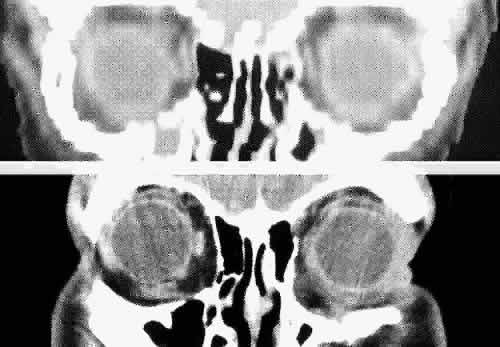
images.1,43–47

The globe is shown in Figure 12. The orbit and periorbital structures are shown in Figures 13 through 16, and the optic canal is shown in Figures 17 through 26. The cavernous sinus and optic chiasm are shown in Figures 27 and 28, and the posterior visual pathway and cranial nerves are shown in Figures 29 through 33.

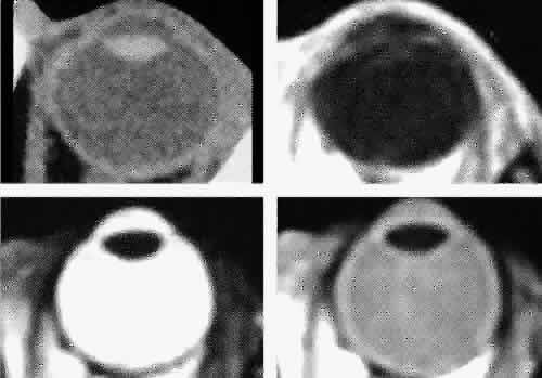
Fig. 12. Axial cuts through the eye. Computed tomography (upper left), T1-weighted magnetic resonance imaging (upper right), T2-weighted magnetic resonance imaging (lower left), proton-density magnetic resonance imaging (lower right).

Fig. 13. Three-dimensional reconstruction of orbit and infraorbital structures (Water's view).

Fig. 14. Three-dimensional reconstruction of orbit (anterior view).

Fig. 15. Three-dimensional reconstruction of orbit and cranial cavity (superior view).

Fig. 16. Three-dimensional bone reconstruction of cranial cavity structures (view from posterior cranial fossa).

Fig. 17. Coronal images through anterior orbit. A. Computed tomography scan. B. T1-weighted magnetic resonance imaging.

Fig. 18. Coronal images through midglobe. A. Computed tomography scan. B. T1-weighted magnetic resonance imaging.

Fig. 19. Coronal images through midorbit posterior to the globe. A. Computed tomography scan.B. T1-weighted magnetic resonance imaging.

Fig. 20. Coronal images through orbital apex. A. Computed tomography scan. B. T1-weighted magnetic resonance imaging. C. Anatomic section of a cadaver head at the level of the orbital apex.

Fig. 21. Coronal images through optic canal. A. Computed tomography scan. B. T1-weighted magnetic resonance imaging.

Fig. 22. Axial images at the level of inferior orbit. A. Computed tomography scan. B. T1-weighted magnetic resonance imaging.

Fig. 23. Axial images at the level of midorbit. A. Computed tomography scan. B. T1-weighted magnetic resonance imaging.

Fig. 24. Axial images at the level of superior orbit. A. Computed tomography scan. B. T1-weighted magnetic resonance imaging.

Fig. 25. Axial images at the level of tendon of the superior oblique. A. Computed tomography scan. B. T1-weighted magnetic resonance imaging.

Fig. 26. T1-weighted magnetic resonance imaging; sagittal image through optic nerve.

Fig. 27. Coronal images through cavernous sinus and optic chiasm. A. T1-weighted magnetic resonance imaging through anterior chiasm. B. Computed tomography image through anterior chiasm. C. Computed tomography image through posterior chiasm. D. Computed tomography image through optic tract.

Fig. 28. Axial computed tomography image with contrast medium through cavernous sinus and pituitary gland.

Fig. 29. A. Axial computed tomography soft tissue image at the level of the base of skull. B. Axial computed tomography bone window image at the level of the base of skull.

Fig. 30. A. Axial T1-weighted image at the level of floor of orbit and trigeminal nerve. B. Axial T1-weighted image at the level of oculomotor nerve.

Fig. 31. Axial T1-weighted image through the cerebral peduncle at the level of oculomotor nerve.

Fig. 32. A. Axial computed tomography soft tissue image at the level of suprasellar cistern. B. Axial computed tomography soft tissue image at the level of thalamus. C. Axial T1-weighted image at the level of thalamus.

Fig. 33. Sagittal T1-weighted image of the brain through the interhemispheric fissure.

GLOBE

Both MRI and CT are limited in their ability to image clearly the normal intraocular structures (see Fig. 12). For the most part this is due to the small size and ultrastructural composition of these structures. The cornea and sclera cannot be differentiated from each other but are quite distinct on both MRI and CT owing to their contrast with both the vitreous and aqueous internally and the orbital fat and, if present, air trapped behind the eyelids externally. The only other readily visible intraocular structure is the lens. On CT this appears uniformly dense and similar in appearance to the sclera. However, on T1-weighted MRI, the external lens capsule can be clearly differentiated from the internal lens structure owing to the presence of a significant number of hydrogen proteins within the central portion of the lens. In addition, the normal choroid, ciliary body, and iris can occasionally be visualized on MRI but not on CT. The normal retina cannot be seen by either technique; neither can the conjunctive, Tenon's capsule, angle structures, or the vessels and nerves penetrating the globe.

ORBIT AND PERIORBITAL STRUCTURES

The bony orbital and periorbital anatomy is best visualized with CT, whereas the soft tissue anatomy can be visualized with either CT or MRI. The orbital cavities are roughly shaped like quadrilateral pyramids parallel to each other medially and lying on one side with their apex facing posteriorly. The widest portion of the orbit is approximately 1.5 cm posterior to the orbital rim (see Fig. 2). On average the adult orbit is 40 to 45 mm deep, with the anterior orbit measuring 40 mm wide and 35 mm high. The interorbital distance in the normal adult is 25 mm. In contrast, the newborn orbit is more rounded, with a width and height of 27 mm, and the orbit of a 7-year-old measures 28 mm high and 33 mm wide.48 The orbital volume is approximately 30 mL, in comparison to the globe, whose diameter of24 mm gives it a volume of 6.5 to 7.0 mL.

The orbital roof is approximately triangular and is composed of the frontal bone anteriorly and the lesser wing of the sphenoid posteriorly. The roof is markedly concave, with the greatest degree of this concavity in the area of the equator of the globe (see Fig. 26). At the anterior and lateral portion of the orbital roof lies the lacrimal gland in the lacrimal fossa (see Figs. 18 and 23). This gland consists of a large orbital portion and a smaller palpebral portion. The orbital portion normally measures 20 × 12 × 5 mm, whereas the palpebral portion is about one third of this size.49 The supraorbital notch is at the junction of the nasal third and the lateral two thirds of the bony orbital margin (see Fig. 1). The trochlea of the superior oblique muscle is located 4 mm posterior to the orbital margin in the medial and anterior portion of the orbital roof (see Figs. 17, 24, and 25). Although usually a cartilaginous structure, it is occasionally partially or wholly ossified. It measures 4 × 6 mm and is firmly attached by connective tissue to the periosteum. The frontal bone portion of the orbital roof is extremely thin and like the orbital floor is subject to so-called blow-in fractures as well as to penetrating injury.50 The posterior portion of the roof is more substantial, measuring 3 mm thick. Except for the anterior portion of the orbit, the intracranial cavity lies directly superior to the orbital cavity (see Fig. 26). The levator muscle and the superior rectus muscle just inferior to it are present along the midportion of the orbital roof for all but its most anterior portion (see Fig. 26). The superior oblique muscle, after it changes direction at the trochlea, is present inferior to the anterior portion of the roof and inserts onto the globe inferior to the superior rectus muscle.

Anteriorly and medially, the frontal sinuses are superior to the orbit and lie between the two plates of the frontal bone. Occasionally, the ethmoid air cells are also found invading the orbital roof. The frontal sinus measures approximately 3 cm high,2.5 cm wide, and 2 cm deep. This is quite variable, and it is not unusual for one sinus to be considerably larger or smaller than the other or even completely absent. The two sinus cavities are separated by a bony septum that is usually deviated to one side. Medially the ethmoid air cells and nasal cavity lie below the frontal sinuses and are separated from them by a thin wall of bone. Superiorly and posteriorly the frontal sinuses are separated from the intracranial cavity and the frontal lobes by the thin frontal bone.

Immediately beneath the central portion of the orbital roof lies the frontal nerve, a branch of the ophthalmic division of the trigeminal nerve (see Fig. 18). Along with the trochlear nerve and lacrimal nerve, another branch of the ophthalmic division of the trigeminal nerve, it enters the orbit through the superior orbital fissure superior to the annular tendinous insertions of the extraocular muscles. The lacrimal nerve enters the orbit medial and superior to the superior orbital vein and travels laterally below the orbital roof and superior to the lateral rectus muscle to enter the lacrimal gland (see Fig. 24). The lacrimal artery arises from the ophthalmic artery lateral to the optic nerve and travels with the distal two thirds of the lacrimal nerve. The supraorbital and supratrochlear arteries branch from the ophthalmic artery superior to the optic nerve, passing medially to the superior rectus and levator muscles to accompany the supraorbital and supratrochlear nerves, the two branches of the frontal nerve, as they pass above the levator muscle. The supraorbital vein and artery accompany the nerve along the anterior two thirds of its course before exiting with it at the supraorbital notch. The other branch of the frontal nerve, the supratrochlear nerve, travels medially after separating from the frontal nerve at approximately the junction of the posterior one third and anterior two thirds of the orbit. The trochlear nerve diverges from the frontal nerve in the posterior orbit, passing medially below the orbital roof and above the levator and superior rectus muscles to enter the superior aspect of the posterior half of the superior oblique muscle.

The orbital floor is similar in shape to the triangular orbital roof and is composed of the maxillary, zygomatic, and palatine bones. Medially, the bony lacrimal canal containing the nasolacrimal duct lies just posterior to the inferior orbital rim (see Fig. 22). At this point the canal is formed by the maxillary and lacrimal bones. Just lateral to the bony canal is the origin of the inferior oblique muscle. Laterally, the floor is separated from the lateral orbital wall by the inferior orbital fissure, which begins lateral and inferior to the optic foremen and near the inferior aspect of the superior orbital fissure. It is approximately 20 mm long, ending 20 mm posterior to the lateral portion of the inferior orbital margin (see Fig. 14). The boundaries of the fissure are the maxillary and palatine bones medially, the greater wing of the sphenoid bone posteriorly, and the zygomatic bone laterally and anteriorly. Inferior to the orbital floor over most of its area is the maxillary sinus (see Figs. 5, 19, and 26). The bone of the floor is 0.5 to 1.0 mm thick, being thinnest at the inferior orbital groove and canal. The fragility of this bone is the reason it is commonly fractured during orbital trauma and the reason for orbital extension of sinus tumors. The ethmoid air cells are occasionally found within the orbital floor medially, and posteriorly there may be a sinus within the orbital portion of the palatine bone.48 The medial rectus muscle runs along the middle aspect of the floor until it inserts into the globe. It is in contact with the floor posteriorly, but anteriorly it is superior to the inferior oblique muscle (see Fig. 19).

The inferior orbital fissure is associated with several important soft tissue and bony structures. The maxillary division of the trigeminal nerve enters the fissure through the foremen rotundum and pterygopalatine fossa, dividing into the infraorbital and zygomatic nerves (see Figs. 20 and 21). This latter nerve separates into the zygomaticofacial and zygomaticotemporal nerves entering the zygomatic bone of the lateral orbital wall through small canals before exiting onto the face. The pterygopalatine fossa is bounded anteriorly by the pterygoid process of the sphenoid bone, the greater wing of the sphenoid, the maxilla, and the palatine bone (see Figs. 21 and 29). In addition to the maxillary division of the trigeminal nerve, it contains the pterygopalatine ganglion and its sensory, parasympathetic, and sympathetic branches and a portion of the maxillary artery. It communicates with the orbit by way of the inferior orbital fissure, the nasal cavity through the sphenopalatine foremen, and with the infratemporal fossa by way of the pterygomaxillary fissure. In addition to the foremen rotundum, sphenopalatine foremen, and pterygomaxillary fissure, the pterygoid and pharyngeal canals also enter into the fossa (see Fig. 29). After leaving the pterygopalatine fossa, the infraorbital nerve travels in the inferior orbital fissure a short distance before turning directly anteriorly into the infraorbital groove and canal within the maxillary bone. Finally it exits from the anterior surface of the bone 4 to 6 mm inferior to the midportion of the inferior orbital rim (see Fig. 19). The infraorbital artery, a terminal branch of the internal maxillary artery, accompanies the nerve along most of its course. Other branches of the maxillary division of the trigeminal nerve include branches to the pterygopalatine ganglion and the posterior, medial, and anterior superior alveolar nerves, which supply sensation to the upper teeth and gums.

The full extent of the orbital roof and floor as well as the superior and inferior rectus muscles and the levator muscle is best evaluated using sagittal views of the orbit (see Figs. 17 through 20, 26). Reconstructed images are generally too crude to provide detailed imaging of these structures. Coronal views of the orbit are excellent for showing the vertical dimension of the lateral and medial orbital walls and the horizontal dimension of the orbital roof and floor. This view is also important for showing the cross-sectional areas of the globe and orbital soft tissue structures, including the muscles, nerves, vessels, and orbital fat.

The lateral wall of the orbit is composed of the zygomatic bone anteriorly and the greater wing of the sphenoid bone posteriorly (see Fig. 14). Although the zygomatic bone also forms a portion of the orbital floor and is separated from the frontal bone and orbital roof by the frontozygomatic suture, posteriorly the sphenoid bone is prominently demarcated from the floor of the orbit by the inferior orbital fissure and from the roof of the orbit by the superior orbital fissure. The lateral wall is triangular and diverges at a 45-degree angle from the medial wall. Posteriorly it is slightly convex; anteriorly it is slightly concave; centrally it is flat. Posteriorly the sphenoid bone portion has a small protuberance of spine that separates the thin superolateral portion of the superior orbital fissure from the wider inferomedial portion. The lateral rectus muscle inserts onto this projection, which is formed in part by the groove containing the superior ophthalmic vein as it passes through the superior orbital fissure. Anteriorly the zygomatic bone has a small bony protuberance, the lateral orbital tubercle. This is just inside the lateral orbital rim and approximately 11 mm below the zygomaticofrontal suture. The levator aponeurosis, lateral canthal ligament, and check ligaments from the lateral rectus muscle insert onto this structure. A small lateral fat pad may also be present in this area.51 Anteriorly, where it is subjected to the greatest stress, the lateral orbital wall is quite thick. In contrast, posteriorly it is quite thin, only 1 mm thick.48 The temporal fossa and temporalis muscle are lateral to the lateral orbital wall for its anterior half, whereas the middle cranial fossa and temporal lobe are lateral to it for its posterior half. The lateral rectus muscle runs along the middle aspect of the wall until it inserts into the globe (see Fig. 23).

The superior orbital fissure separates the orbital roof from the lateral orbital wall and the lesser and greater wings of the sphenoid bone (see Figs. 13 and 14). The common tendinous ring (annulus of Zinn) of the extraocular muscles and the spine for the insertion of the lateral rectus muscle separates the fissure into a thin superolateral portion and a wide inferomedial portion (see Fig. 21). The fissure is approximately 22 mm long, and its superior end is 30 to 40 mm from the frontozygomatic suture.48 Directly posterior to the fissure are the middle cranial fossa and temporal lobe. Passing through the superior portion of the fissure above the tendinous ring are the lacrimal (cranial nerve V), frontal (cranial nerve V), and trochlear (cranial nerve IV) nerves, the superior ophthalmic vein, and the recurrent lacrimal artery. Passing within the ring are the superior division of the oculomotor nerve (cranial nerve III) and the abducens nerve (cranial nerve VI) laterally, the nasociliary nerve (cranial nerve V) and the inferior division of the oculomotor nerve medially, and the sympathetic root of the ciliary ganglion and the inferior ophthalmic vein, which on occasion may pass below the ring. The tendinous insertions of the lateral and inferior rectus muscles form the superior, lateral, and inferior portions of the ring in the area of the superior orbital fissure. There is no muscle tendon medial to the fissure. The medial border of the fissure is formed by a strut of bone from the lesser wing of the sphenoid bone, which separates it from the optic canal.

The medial wall of the orbit is formed by four bones: the frontal process of the maxillary bone, the lacrimal bone, the orbital portion of the ethmoid bone, and a small portion of the lesser wing of the sphenoid bone. Generally, this wall is parallel to the sagittal plane and is somewhat quadrilateral, unlike the other walls of the orbit. Superiorly and inferiorly this wall blends into the orbital roof and floor (see Fig. 14). Anteriorly the wall contains the lacrimal sac within the lacrimal fossa. This is formed by portions of the lacrimal and maxillary bones. The fossa is bounded anteriorly by the anterior lacrimal crest and posteriorly by the posterior lacrimal crest. The anterior lacrimal crest blends into the inferior orbital rim. Inferiorly the lacrimal fossa turns into the bony nasolacrimal canal, which exits beneath the inferior turbinate bone approximately 4 cm posterior to the opening of the nares (see Figs. 14 and 17). This structure is bounded by parts of the lacrimal, maxillary, and inferior turbinate bones. The fossa measures approximately 14 mm vertically and 5 mm anteroposteriorly, whereas the canal measures approximately 15 mm vertically.48 Medial to the lacrimal fossa, the anterior portion of the ethmoid air cells is present superiorly as well as the middle meatus of the nasal cavity inferiorly. Medial to the bony nasolacrimal canal is the middle meatus and inferior turbinate superiorly and the inferior meatus inferiorly.

The ethmoid portion of the medial wall contains the thinnest bone of the orbit (lamina papyracea). It is translucent to light and is only 0.2 to 0.4 thick (see Fig. 23).48 Because of its thinness, this area of the medial orbital wall is frequently prone to fracture. Anteriorly the medial wall is adjacent to the nasal cavity, middle turbinate, lateral wall of the nose, and the ethmoid sinus cavity. At its far posterior aspect the wall is adjacent laterally to the sphenoid sinus and medially to the optic canal (see Fig. 3). The superior oblique muscle runs along the superior aspect of the wall for most of its length before changing direction at the trochlea. The medial rectus muscle runs along the middle aspect of the wall until it inserts into the globe. The cribriform plate of the ethmoid bone is present medial to the superior aspect of the medial orbital wall at the point where the frontal and ethmoid bones join (see Figs. 5 and 24). Superior to the midportion of the cribriform plate and midway between the two medial orbital walls is a vertical portion of the ethmoid called the crista galli. Inferior to the cribriform plate and directly below the crista galli is the portion of the ethmoid bone forming the bony vertical aspect of the nasal septum (vomer bone). The anterior and posterior ethmoidal canals, which contain the posterior and anterior ethmoidal arteries, both branches of the ophthalmic artery, are present at the junction of the medial orbital wall and the orbital roof. The anterior canal is about 25 mm posterior to the anterior lacrimal crest, whereas the posterior canal is about 13 mm posterior to the anterior canal and about 8 mm anterior to the orbital opening of the optic canal.

The optic canal is contained entirely within the lesser wing of the sphenoid bone, leading from the middle cranial fossa to the orbit (see Figs. 3 and 21). The anterior opening of the canal measures approximately 6 mm vertically by 5 mm horizontally and is larger than the posterior opening, which is wider horizontally than vertically.48 Anteriorly, the canals form a 36-degree angle with the sagittal plane and are about 30 mm apart. Posteriorly, the canals form a 90-degree angle if they are invisibly extended to the dorsum sellae. Intracranially, they are about 20 to 25 mm apart. The canals vary in length from 5 to 12 mm. Medial to the optic canal is the anterior portion of the sphenoid sinus and the posterior portion of the ethmoid sinus (see Fig. 3). Optic nerve injury can occur during sinus surgery when the lateral walls of these sinuses are inadvertently violated. Superior to the canal is the gyrus rectus of the frontal lobe and the olfactory tracts (see Fig. 21). The canal transmits the optic nerve with its meningeal covering, sympathetic nerve fibers, and the ophthalmic artery. The intraorbital portion of the optic nerve is serpentine and 25 to 30 mm long. The intracanalicular nerve is 6 to 10 mm long, and the intracranial portion is 10 to 15 mm long. The ophthalmic artery is initially below and then lateral to the nerve as it exits the canal (see Figs. 23 and 26). It then moves superiorly between the optic nerve and superior rectus muscle to travel medially between the medial rectus and superior oblique muscles before ending in its terminal branches, the supratrochlear and dorsal nasal arteries. The medial rectus muscle inserts into the annulus of Zinn medial to the optic nerve, whereas the superior rectus muscle inserts into the annulus superior to the nerve. Because of the close approximation of these two muscles to the nerve, movement of these muscles can be painful in cases of retrobulbar neuritis. The levator muscle inserts into the annulus superior to the superior rectus muscle, and the suerior oblique muscle inserts into the annulus medial and somewhat superior to the medial rectus muscle. As noted previously, the lateral and inferior rectus muscles insert into the common tendinous ring in the area of the superior orbital fissure, lateral to the optic canal. Within the orbit the muscles are interconnected through intermuscular septa, which also extend to insert into the periorbita.52

INTRACRANIAL STRUCTURES

After exiting the optic canals, the optic nerves enter an area known as the cisterna basalis. This region is almost completely surrounded by the intracranial portions of the sphenoid bone, being bounded anteriorly by the tuberculum sellae, anterior cranial fossa, and anterior clinoid processes; posteriorly by the clivus, dorsum sellae, and posterior clinoid processes; inferiorly by the sella turcica; laterally by the cavernous sinuses; and superiorly by the frontal lobe and third ventricle (see Figs. 2, 26, and 27). The tentorium cerebelli, a transaxial fold of aura separating the cerebellum from the posterior portion of the cerebral hemispheres, extends from the petrous portion of the sphenoid bone and anterior clinoid processes to the straight sinus and falx cerebri separating the cerebral hemispheres in the sagittal plane. The free edge of the tentorium is superior to the cavernous sinus.

The diaphragma sellae connects the clinoid processes, forming a roof over the sella turcica, which contains the hypophysis (pituitary gland). The hypophyseal stalk extends through an opening in the diaphragma sella, posterior to the optic chiasm, and connects to the hypothalamus and floor of the third ventricle. In this area the posterior portion of the chiasm is separated from the ventricle by the thin plate of hypothalamus with which it is in direct contact. Inferior to the hypophysis are the sphenoid sinuses. Laterally are the cavernous sinuses, with the intracavernous portions of the internal carotid artery in close approximation to the gland. The intercavernous sinuses or circular sinus connecting the two cavernous sinuses are both directly above and below.

The optic nerves converge at an angle of approximately 90 degrees to join at the optic chiasm. The optic tracts diverge from the chiasm posteriorly. The chiasm measures approximately 12 mm transversely and 8 mm anteroposteriorly.48 It lies at an oblique angle of 45 degrees, with its posterior portion higher than its anterior portion (see Figs. 26 and 33).53 It lies directly above the diaphragma sella, being separated from it by 5 to 10 mm. Portions of the interpeduncular and chiasmatic cisterns are inferior and posterior to the chiasm. The former contains the circle of Willis, which is superior to the pituitary fossa. In most cases (79%), the posterior aspect of the chiasm is directly over the dorsum sellae. However, in 12% of cases it is over the diaphragma sellae, in 5% it is over the tuberculum sellae, and in 1% to 2% it is behind the dorsum sellae.53 The close approximation to the optic nerves, chiasm, and optic tracts of the meninges covering the bony structures, cisterns, and venous sinuses surrounding the cisterna basalis is the reason meningiomas in this area frequently result in visual symptomatology. The extracavernous portion of the internal carotid artery is lateral to the chiasm along with the anterior perforated substance of the frontal lobe. Anteriorly, the chiasm is bounded by the anterior cerebral arteries and the anterior communicating artery. Posteriorly, it is bounded by a portion of the third ventricle and beyond that the tuber cinereum, a thin plate of gray matter, connected superiorly to the mammillary bodies and separated from the infundibulum by the infundibular cavity of the third ventricle. Inferoposteriorly within the interpeduncular cistern are the basilar, posterior cerebral, and posterior communicating arteries (see Fig. 33). The oculomotor nerve (cranial nerve III) is also posterior and inferior as it passes from the midbrain under the posterior cerebral artery and above the superior cerebellar artery before entering the cavernous sinus. Also sitated posteriorly are the pons and cerebral peduncles, which are separated from the dorsum sellae and clivus by the interpeduncular cistern. Aneurysms involving the posterior cerebral and communicating arteries frequently affect the third nerve and posterior aspect of the chiasm, whereas aneurysms involving the anterior cerebral and communicating arteries may affect the anterior portion of the chiasm. The blood supply to the chiasm is from the anterior cerebral and internal carotid arteries.

The cavernous sinuses lie on either side of the pituitary fossa in the middle cranial fossa, lateral and superior to the sphenoid sinus. These endothelial-lined structures extend from the superior orbital fissure to the apex of the petrous bone and are completely covered by dura (see Fig. 27). The sinuses receive venous blood from the superior and inferior ophthalmic veins, cerebral veins, and the sphenoparietal sinus. They have connections with the transverse sinus, pterygoid plexus, angular and facial veins, and the contralateral sinus through the intercavernous sinuses. They drain into the inferior petrosal sinus and internal jugular vein. Several structures pass through each sinus. In the lateral wall of the sinus, starting superiorly and going inferiorly, are the oculomotor nerve (cranial nerve III), trochlear nerve (cranial nerve IV), the ophthalmic division of the trigeminal nerve (cranial nerve V), and the maxillary division of the trigeminal nerve (see Fig. 27). In the anterior portion of the sinus, the trochlear nerve is above the oculomotor nerve. The carotid artery and abducens nerve (cranial nerve VI) are suspended within the sinus by fibrous septations. The abducens nerve is in the midportion of the sinus just medial to the ophthalmic division of the trigeminal nerve. The internal carotid artery travels upward through the sinus after it passes through the carotid canal and foremen lacerum in the petrous portion of the temporal bone. Sympathetic nerve fibers from the superior cervical ganglion travel with it. Anteriorly, before entering the cavernous sinus, the artery is separated from the trigeminal ganglion by a thin plate of bone and by a fibrous membrane. Within the cavernous sinus, the artery first travelsposteriorly toward the posterior clinoid process. It then turns anteriorly in the medial aspect of the sinus and curves to travel upward toward the anterior clinoid process, finally perforating the sinus. After passing between the optic and oculomotor nerves, it turns toward the anterior perforted substance and divides into its terminal branches, the anterior and middle cerebral, posterior communicating, and anterior choroidal arteries (see Fig. 20). The ophthalmic artery arises from the carotid as it leaves the cavernous sinus on the medial side of the anterior clinoid process. It travels through the optic canal inferior and lateral to the optic nerve before entering the orbit, where it rotates to a position superior and medial to the nerve.

The oculomotor nerve nuclei arise in the midbrain and consist of a paired group of motor cells in the form of a V, measuring approximately 10 mm long.53 The nuclei are just ventral to the central gray matter of the mesencephalon that surrounds the cerebral aqueduct. Superiorly the nuclei extend almost as far as the floor of the third ventricle; inferiorly they end just below the superior colliculus. The medial longitudinal fasciculus is ventral and lateral to these nuclei. Inferiorly the nuclei blend with the trochlear nerve nuclei. The oculomotor nerve fibers travel ventrally after leaving the nuclei, passing through the brain stem. They successively cross the medial longitudinal fasciculus, the red nucleus, the substantia nigra, and the anterior border of the pons to exit as paired nerve trunks in the interpeduncular fossa at the angle of the pons and cerebral peduncle. The nerve then travels anteriorly and laterally below the posterior cerebral and above the superior cerebellar arteries to enter the cavernous sinus. As it emerges from the cavernous sinus, it passes lateral to the carotid artery near the uncus of the temporal lobe to enter the orbit through the superior orbital fissure. It then divides into a superior branch, innervating the levator and superior rectus muscles, and an inferior branch, innervating the medial and inferior rectus and the inferior oblique muscles (see Fig. 20).

Sympathetic fibers from the carotid plexus travel with the superior branch of the third nerve to innervate Muller's muscle. After synapsing in the pretectal nuclei near the superior colliculi, the parasympathetic fibers for pupillary constriction travel in the superior peripheral portion of the nerve as it leaves the brain stem. They then follow the inferior nerve branch to the inferior oblique muscle, leaving it to synapse in the ciliary ganglion. This structure, measuring about 2 × 1 mm, is located in the posterolateral portion of the orbit between the optic nerve and lateral rectus muscle and 1 cm anterior to the optic foramen. It is adjacent to the nerve and near the ophthalmic artery. Both sympathetic fibers to the pupil and ocular blood vessels and sensory fibers to the cornea, iris, and ciliary body pass through this ganglion.

The paired nuclei for the trochlear nerve are located just below the oculomotor nerve nuclei just ventral to the central gray substance in the mesencephalon. Like the oculomotor nerve nuclei, they are ventral and lateral to the cerebral aqueduct and dorsal and medial to the medial longitudinal fasciculus. They are on the same level as the superior aspect of the inferior colliculus. The nerve fibers arising from these nuclei travel dorsally and laterally around the central gray substance and cross dorsally to this structure before exiting the brain stem as nerve roots near the inferior aspect of the inferior colliculi. This is the only cranial nerve to exit from the dorsal surface of the brain stem, and it has the longest intracranial course (75 mm) of any cranial nerve.48 The nerve then courses anteriorly and ventrally around the superior portion of the cerebral peduncles to the anterior aspect of the brain stem. It proceeds forward between the posterior cerebral and superior cerebellar arteries, medial and superior to the trigeminal nerve and below the free edge of the tentorium cerebelli, to enter the cavernous sinus below the oculomotor nerve.

The motor and sensory nuclei of the trigeminal nerve are in the dorsal part of the pons, lateral and ventral to the fourth ventricle. The sensory nuclei are a superior continuation of the sensory column of the spinal cord and are present throughout the entire brain stem. The motor nuclei are ventral and medial to the superior cerebellar peduncles and lateral to the nuclei of the abducens nerves and nuclei and fibers of the facial nerve. Proprioceptive fibers arise from the main sensory (mesencephalic) nuclei located in the superior aspect of the pons near the superior cerebral peduncle and lateral to the cerebral aqueduct. Motor fibers arise from the pontine area medial to the sensory nuclei and closer to the fourth ventricle. The spinal nuclei are the location for thermal and tactile sensation. The fibers from the mandibular division go to the most superior portion of these nuclei, those from the maxillary division to the middle portion, and those from the ophthalmic division to the most inferior portion. The motor and sensory nerve fibers travel through the middle cerebral peduncle to exit the pons near the middle of its lateral aspect (see Fig. 30). The nerve roots then travel approximately 1 cm anteriorly and slightly superiorly in the pontine cistern toward a slight depression in the petrous portion of the temporal bone lateral to the oculomotor, trochlear, and abducens nerves. The free edge of the tentorium and the cerebellum are above the nerve fibers, and the facial and vestibulocochlear nerves are lateral and inferior to them.

The nerve fibers enter the trigeminal (gasserian) ganglion, which is located in Meckel's cave, a aural pocket lateral to the cavernous sinus and carotid artery in a depression formed at the apex of the petrous portion of the temporal bone. Below the ganglion are the greater and lesser petrosal nerves and the foremen lacerum containing the carotid artery. Laterally is the foremen spinosum, which transmits the middle meningeal artery. Superiorly are the uncus and temporal lobe. The motor branch of the nerve travels below the ganglion to exit with the mandibular division of the nerve through the foremen ovale. The ganglion measures approximately 1 × 2 cm and is bean-shaped.48 The ophthalmic division of the nerve leaves the ganglion from its anterior and superior aspect, passing through the lateral aspect of the cavernous sinus within its own separate aural sheath. It passes into the orbit through the superior orbital fissure with sympathetic fibers from the carotid plexus. As described earlier, in the orbit it divides into three branches, the frontal, lacrimal, and nasociliary nerves. The ophthalmic division supplies sensation to the eye, conjunctive, cornea, lacrimal gland, a portion of the nasal and sinus mucosa and skin of the eyelids, forehead, and nose. The maxillary division of the nerve leaves the ganglion positioned between the two other divisions. It travels in the inferior aspect of the cavernous sinus close to the lateral wall and below the ophthalmic division before exiting the cranial cavity through the foremen rotundum, crossing the pterygopalatine fossa, and entering the infraorbital fissure. It supplies sensation to portions of the aura, midface, lower eyelid, side of the nose, upper lip, and mucosa of the maxillary sinus, soft palate, upper gums, hard and soft palate, and nasopharynx and to the upper teeth.

The paired motor nuclei of the abducens nerves are located in the floor of the fourth ventricle on either side of the midline. The fibers of the facial nerves course around these nuclei, forming a small elevation in the floor of the ventricle called the facial colliculus. The medial longitudinal fasciculus is medial to the nuclei, and the vestibular nuclei are lateral to the nuclei and the facial nerve fibers. The abducens nerve fibers travel ventrally without decussating through the tegmentum and pons. The nerve roots exit the lower portion of the pons on either side of the midline. They course forward, upward, and somewhat laterally in the middle cranial fossa toward the petrous process of the temporal bone. The two nerve roots are approximately 1 cm apart at their origin. The basilar artery is medial to them and the origin of the facial nerve is lateral to them. The abducens nerves are crossed near their origin by the anteroinferior cerebellar arteries. They travel superiorly between the pons and basilar portion of the occipital bone to reach the petrous process of the temporal bone about 2 cm below and lateral to the posterior clinoid process and slightly medial or posterior to the inferior petrosal sinus.48 Each nerve root then passes forward and laterally over the petrous portion of the temporal bone in a small groove (Dorello's canal) to which it is held by the petrosphenoidal (Gruber's) ligament. It then passes through the aura to enter the cavernous sinus together with the inferior petrosal sinus. In the sinus the nerve courses around the lateral aspect of the internal carotid artery. It lies in the sinus in a more medial position than the other nerves and within its own separate sheath. The nerve enters the orbit through the annulus of Zinn below the oculomotor nerve.

The nuclei of the facial nerve are located deep in the reticular formation of the brain stem ventral and lateral to the abducens nuclei. The fibers from the nuclei travel dorsally toward the fourth ventricle and circle laterally around the abducens nuclei. They then turn ventrally again to exit the pons between the olive and the inferior cerebellar peduncle. At this point the nerve is medial to the auditory nerve and lateral to the abducens nerve. The nervus intermedius, a portion of the facial nerve carrying sensory fibers for taste as well as parasympathetic fibers, lies on the lateral side of the facial nerve. The nervus intermedius and facial and auditory nerves travel together anteriorly and laterally into the internal auditory meatus. The facial nerve and nervus intermedius separate from the auditory nerve and enter the facial canal in the petrous portion of the temporal bone. Initially the nerve continues its lateral course between the cochlea and semicircular canals. Near the tympanic cavity it turns posteriorly, running in the medial wall of the cavity. At this point the frontal nerve merges into the geniculate ganglion. From this structure the greater petrosal, vidian, and lesser petrosal nerves and the afferent division of the nervus intermedius arise. The nerve then dips into the mastoid air cells and exits from the stylomastoid foramen. At this point the posterior auricular, digastric, and stylohyoid branches of the nerve arise. It then enters the substance of the parotid gland, where its various facial branches, the temporal, zygomatic, buccal, mandibular, and cervical divisions, arise.

The medial longitudinal fasciculus is close to the midline just ventral to the aqueduct and fourth ventricle. It extends from the pons to the medulla and into the spinal cord. This tract coordinates the nuclei of the oculomotor, trochlear, and abducens nerves to allow conjugate movement of the eyes. In addition, it integrates these movements with impulses from the vestibular apparatus as well as with motor movements of the neck. It is particularly important in relaying impulses between the medial rectus muscle and the contralateral pontine gaze center.

The optic tracts extend posteriorly and laterally from the chiasm, passing around the basilar artery, mammillary bodies, and cerebral peduncle and between the anterior perforated substance and tuber cinereum. Each tract is attached to the lateral surface of the peduncle just lateral to the hypothalamic nuclei and third ventricle as well as the internal capsule.48 The anterior choroidal and posterior cerebral arteries run parallel and across the tracts. The tracts ascend slightly as they move laterally around the peduncle crossing the pyramidal tracts. Posteriorly the globus pallidus is above and the hippocampus is below the tracts, which come very close to the inferior horn of the lateral ventricle. The tracts and the afferent visual fibers then pass into the lateral geniculate bodies (see Fig. 31). These triangular areas of the thalamus are located inferior and lateral to the major portions of the thalamus. Medial to the lateral geniculate body is the medial geniculate body and portions of the internal capsule. The lateral geniculate body is adjacent to the hippocampal convolution inferiorly, the pulvinar superiorly, and the inferior horn of the lateral ventricle posteriorly. As the optic tracts enter the lateral geniculate body, they are just lateral and adjacent to the major motor tracts, including the pyramidal tracts. The optic tract enters the lateral geniculate anteriorly and ventrally to synapse with the neuronal components in its various layers. The blood supply to this structure is from the anterior choroidal artery anteriorly and the posterior cerebral artery posteriorly. The optic radiations exit from its dorsal surface. The superior colliculi, situated on the dorsal aspect of the midbrain, are connected to the lateral geniculate bodies by the superior brachium. This structure transmits afferent pupillary fibers to the pretectal region and afferent fibers from the optic tract to the superior colliculi for reflex control of the ocular muscles.

After leaving the lateral geniculate bodies, the optic radiations, also called the geniculocalcarine radiations, turn anteriorly and then laterally at the optic peduncle to bypass the lateral ventricle (see Fig. 32). The posterior and medial aspect of this tract, representing fibers from the upper portions of the retina and macula, proceeds directly through the parietal lobe to the occipital cortex, terminating superior to the calcarine fissure. The anterior and lateral aspect of this tract, representing fibers from the lower portions of the retina and macula, turns anteriorly and traverses the temporal horn of the lateral ventricle before proceeding to the occipital cortex terminating inferior to the calcarine fissure. These fibers pass through the temporal lobe. Their most anterior position is called Meyer's loop. Injury to this area results in a superior homonymous quadrantic hemianopia. Just posterior and lateral to the internal capsule as the optic radiations proceed posteriorly, they cross the temporal isthmus. This is an area approximately 1.5 cm in diameter where visual, somesthetic, motor, speech, and intracerebral association pathways are in close proximity.53 Lesions in this area, often resulting from anterior choroidal artery occlusion, are associated with hemianopia, aphasia, numbness in the opposite extremities, and motor weakness of the leg. The blood supply to the optic radiations is from the anterior choroidal artery anteriorly, the middle cerebral artery in its middle portion, and the posterior cerebral artery posteriorly.

Back to Top
REFERENCES

1. Zonneveld FW, Koornneef L, Hillen B, de Slegte RGM: Normal direct multiplanar CT anatomy of the orbit with correlative anatomic cryosections. Radiol Clin North Am 25:381, 1987

2. Zonneveld FW, Vijverberg GP: The relationship between slice thickness and image quality in CT. Medicamundi 29:104, 1984

3. Multislice spiral/helical computed tomography: physical principles and instrumentation. In: Seerman E, ed: Computed tomography: physical principles, clinical applica-tions, and quality control, 2d ed, pp 201–265. Philadelphia, Lippincott, Williams and Wilkins, 2001

4. Hammerschlag SB, Wolpert SM, Carter B: Computed coronal tomography. Radiology 120:219, 1976

5. Wolf BS, Nakagawa H, Staulcup PH: Feasibility of coronal views in computed scanning of the head. Radiology 120:217, 1976

6. Zonneveld FW, Koornneef L: Patient positioning for direct sagittal CT of the orbit parallel to the optic nerve. Radiology 158:547, 1986

7. Bluemm R: Direct sagittal positional computed tomography of the head. Neuroradiology 22:199, 1982

8. Stytz MR, Frieder O: Three-dimensional medical imaging modalities: An overview. Crit Rev Biomed Eng 18:1, 1990

9. Slamovits TL, Gardner TA: Neuroimaging in neuroophthalmology. Ophthalmology 96:555, 1989

10. Council on Scientific Affairs: Magnetic resonance imaging of the head and neck region: Present status and future potential. JAMA 260:3313, 1988

11. DeMarco JK, Bilaniuk LT: Magnetic resonance imaging: Technical aspects. In Newton TH, Bilaniuk LT, eds: Radiology of the Eye and Orbit, pp 1.1–1.14. New York, Raven Press, 1990

12. Nicolle D, Ethier R, Peters T: Clinical application of multiplanar computerized tomography of the orbit. Can J Ophthalmol 16:124, 1981

13. Baker HJ: The clinical usefulness of routine coronal and sagittal reconstructions in cranial computed tomography. Radiology 140:1, 1981

14. Rothman S, Geehr R, Kier E, Hoffman H: Multiplanar reconstruction as an aid in CT diagnosis. Neuroradiology 16:596, 1978

15. Ball JB Jr, Towbin RB, Staton RE, Cowdrey KE: Direct sagittal computed tomography of the head. Radiology 155:822, 1985

16. Napel S: Principle and techniques of 3D spiral CT angiography. In: Fishman EK, Jeffrey BR Jr, eds: Spiral CT: Principles, Techniques, and Clinical Applications, 2d ed, pp 339–60. Philadelphia, Lippincott-Raven, 1998

17. Computed tomography angiography: technical considerations. In: Seerman E, ed: Computed Tomography: Physical Principles, Clinical Applications, and Quality Control, 2d ed, pp 303–313. Philadelphia, Lippincott Williams and Wilkins, 2001

18. Bradley WG Jr: Magnetic resonance imaging in the central nervous system: Comparison with computed tomography. Magnetic Resonance Annu 81, 1986

19. Breger R, Kneeland JB: Basic physics of magnetic resonance imaging. In Daniels DL, Haughton VM, Naidich TP, eds: Cranial and Spinal Magnetic Resonance Imaging, pp 1–20. New York, Raven Press, 1987

20. Elliott DO: Magnetic resonance imaging fundamentalsand system performance. Radiol Clin North Am 25:409,1987

21. Hawkes R, Holland G, Moore W, Worthington B: Nuclear magnetic resonance (NMR tomography) of the brain: A preliminary clinical assessment with demonstration of pathology. J Comput Assist Tomogr 4:577, 1980

22. Holland G, Hawkes R, Moore W: Nuclear magnetic resonance (NMR tomography) of the brain: Coronal and sagittal sections. J Comput Assist Tomogr 4:429, 1980

23. Bradley W, Crooks L, Newton T: Physical principles of NMR. In Newton T, Potts D, eds: Modern Neuroradiology, pp 15–61. San Francisco, Clavadel Press, 1983

24. Hahn E: Spin echoes. Phys Rev 80:580, 1950

25. Daniels DL, Haughton VM: Guidelines to interpreting cranial MR images. In Daniels DL, Haughton VM, eds: Cranial and Spinal Magnetic Resonance Imaging, pp 5–20. New York, Raven Press, 1987

26. Wehrli FW, Kanal E: Orbital imaging: Factors determining magnetic resonance imaging appearance. Radiol Clin North Am 25:419, 1987

27. Atlas S, Grossman R, Hackney D et al: STIR MR imaging of the orbit. Am J Neuroradiol 9:969, 1988

28. Schenck JF, Hart HR Jr, Foster TH et al: Improved MR imaging of the orbit at 1. 5T with surface coils. Am J Neuroradiol 6:193, 1985

29. Simon J, Szumowski J, Totterman S et al: Fat-suppression MR imaging of the orbit. Am J Neuroradiol 9:961, 198

30. Mirvis S, Borg U, Belzberg H: MR imaging of ventilatordependent patients: Preliminary experience. Am J Roentgenol 149:845, 1987

31. New PF, Rosen BR, Brady TJ et al: Potential hazards and artifacts of ferromagnetic and nonferromagnetic surgical and dental material and devices in nuclear magnetic resonance imaging. Radiology 147:139, 1983

32. Shellock F: MR imaging of metallic implants and materials:A compilation of the literature. Am J Roentgenol 151:811,1988

33. Kelley W, Paglen G, Pearson J et al: Ferromagnetism of intraocular foreign body causes unilateral blindness after MR study. Am J Neuroradiol 7:243, 1986

34. Clark J, Kelly W: Common artifacts encountered in magnetic resonance imaging. Radiol Clin North Am 26:893, 1988

35. Pusey E, Lufkin RB, Brown RK et al: Magnetic resonance imaging artifacts: Mechanism and clinical significance. RadioGraphics 6:891, 1986

36. Bradley WG, Waluch V: Blood flow magnetic resonance imaging. Radiology 154:443, 1985

37. Masaryk TJ, Lewin JS, Laub G: Magnetic resonance angiography. In Stark DD, Bradley WG, eds: Magnetic Resonance Imaging, ed 2, pp 299–334. St. Louis, Mosby, 1992

38. Axel L: blood flow effects in magnetic resonance imaging. Am J Roentgenol 1157, 1984

39. Masaryk TJ, Perl J II, Dagirmanjian A et al: Magnetic resonance angiography: neuroradiological applications. In Stark DD, Bradley WG, eds: Magnetic Resonance Imaging, ed 3, pp 1277–1316. St. Louis, Mosby, 1999

40. Blatter DD, Parker DL, Ahn SS et al: Cerebral MR angiography with multiple overlapping thin slab acquisition. II. Early clinical experience. Radiology 183:379, 1992

41. Hamed LM, Silberg J, Silberg M el al: Magnetic resonance angiography of vascular lesions causing neuroanatomic deficits. Surv Ophthalmol 37:425, 1993

42. Ettl A, Kamer J, Daxer A et al: High-resolution magnetic resonance imaging of neurovascular orbital anatomy. Ophthalmology 104:869, 1997

43. Bilaniuk LT, Atlas SW, Zimmerman RA: Magnetic resonance imaging of the orbit. Raiol Clin North Am 25:509, 1987

44. Langer BG, Mafee MF, Pollack S et al: MRI of the nor-mal orbit and optic pathway. Radiol Clin North Am 25:429,1987

45. Unsold R, deGroot J: Computed tomography: Orbitalanatomy. In Newton TH, Bilaniuk LT, eds: Radiology ofthe Eye and Orbit, pp 8.1–8.16. New York, Raven Press,1990

46. Mafee M: Magnetic resonance imaging: Ocular anatomy. In Newton TH, Bilaniuk LT, eds: Radiology of the Eye and Orbit, pp i.1–2.4. New York, Raven Press, 1990

47. Daniels DL, Haughton VM, Naidich TP: Cranial and Spinal Magnetic Resonance Imaging: An Atlas and Guide. New York, Raven Press, 1987

48. Warwick R: Eugene Wolff's Anatomy of the Eye and Orbit, 7th ed. Philadelphia, WB Saunders, 1976

49. Whitnall S: The Anatomy of the Human Orbit and Accessory Organs of Vision, 2nd ed. London, Oxford University Press, 1932

50. Karesh J, Kelman S, Chirico P, Mirvis S: Orbital roof “blow-in” fractures. Ophthalmic Plast Recon Surg 7:77, 1991

51. Zide BM, Jelks GW: Surgical Anatomy of the Orbit. New York, Raven Press, 1985

52. Koornneef L: Orbital connective tissue. In Duane TD, ed: Biomedical Foundations of Ophthalmology, vol I, chap 32. Philadelphia, JB Lippincott, 1982

53. Cogan D: Neurology of the Visual System. Springfield, IL, Charles C. Thomas, 1966

Back to Top