Chapter 65
Basic Statistics and Epidemiology for Ophthalmologists
ANDREW F. SMITH
Main Menu   Table Of Contents

Search

POPULATION AND SAMPLES
INDUCTIVE VERSUS DEDUCTIVE STATISTICS
TYPES OF VARIABLES
FREQUENCY DISTRIBUTIONS
MEASURES OF CENTRAL TENDENCY
MEASURES OF DISPERSION
MEAN DEVIATION
VARIANCE
PROPERTIES OF THE NORMAL DISTRIBUTION OR NORMAL CURVE
PARAMETRIC STATISTICS
CONFIDENCE INTERVALS
TESTING HYPOTHESIS WITH THE “TEST” STATISTIC
NONPARAMETRIC STATISTICS
INTERPRETING A DIAGNOSTIC TEST
AN OVERVIEW OF STUDY DESIGNS
CLINICAL TRIALS
OBSERVATIONAL STUDIES
RATES
RELATIVE RISK RATIOS
ODDS RATIO
SAMPLE SIZE
REFERENCES

The focus of this chapter is to explore and explain the main mathematic concepts used to describe and interpret the complex range of biologic, environmental, and other factors that impact on ocular morbidity (disease) and mortality (death). At a minimum, this chapter increases the ophthalmologist's level of understanding of statistical and epidemiologic concepts and terminology used in the design, analysis, and interpretation of ophthalmic studies and data. At a maximum, this increased knowledge should result in the development of new, more efficacious, cost-effective, and evidence-based treatments and interventions that promote healthy eyesight, the prevention of vision loss, and, where possible, the reversal of blindness. The material is presented in short, discreet sections beginning with the fundamental concepts and proceeding to more advanced concepts.
Back to Top
POPULATION AND SAMPLES
A fundamental principle of statistics resides in being able to draw conclusions about a given population from a representative sample selected at random. In this respect, populations can either be finite, such as the number of operating theaters available at any one time, or infinite in the sense that one can sum all the possible outcomes arising from successive tosses of a coin, be it heads or tails.
Back to Top
INDUCTIVE VERSUS DEDUCTIVE STATISTICS
Theoretically, statistics can be divided into two broad camps, namely, inductive and deductive statistics. Inductive or inferential statistics relies on the use of probabilities to measure the potential that a given event will or will not take place. By contrast, deductive or descriptive statistics presents the data as they are rather than drawing conclusions from them.
Back to Top
TYPES OF VARIABLES
A variable may be thought of as a letter or symbol that can take on a predetermined set of values, which are denoted by the domain of a variable. Thus, a constant is a variable for which there is only one value. Continuous variables can assume any value between two other given values, such as 0 to 1, or 90 to 100, and all values in between. A discreet variable, by contrast, can move only from one value to the next in accordance with a set pattern. In addition, four broad types of variables can be defined. Nominal and ordinal variables refer to specific categories and require the use of “nonparametric” statistics to analyze them. By contrast, interval and ratio variables provide actual measurements and, as such, require the use of “parametric” statistical methods to be analyzed (Table 1).


TABLE 1. Types of Variables


TypeExample
Qualitative 
NominalReligion, gender
OrdinalStage of disease
Quantitative 
Interval0–1
RatioPulse
DependentIris melanoma
IndependentChemotherapy vs radiation therapy


Back to Top
FREQUENCY DISTRIBUTIONS
To organize raw data into a more meaningful format, statisticians often sort data into various classes or categories. The number of cases within a particular class is called the class frequency, and the arrangement of all of the classes or categories into a table format yields the frequency distribution for that particular set of data. In Table 2, for example, 30 patients have been grouped according to their intraocular pressure readings into seven categories. The resulting distribution of the number of patients in each of the intraocular pressure categories is called a frequency distribution. The relative frequency distribution for the same group of patients can be found by adding up all of the patients in each intraocular pressure category and dividing by the total number of patients examined, in this case, 30. Often, the relative frequency distribution is presented as the percentage of the total data contained within a given frequency. Last in this regard, to determine what percentage of the total amount of data is contained among any of the categories, the number of cases in such frequencies is summed, along with the relevant percentages, until all of the categories have been added up. These two frequency distributions are known as the cumulative frequency and cumulative percentage distributions, respectively (see Table 2).


TABLE 2. Frequency Distributions


Class (IOP mm Hg)Frequency (No. of Patients)Relative PercentageCumulative FrequencyCumulative Percentage
0–413.313.3
5–926.639.9
10–14310.0619.9
15–191033.31653.2
20–24826.62479.8
25–29413.32893.4
30+26.630100.0
Total30100.0  

IOP, intraocular pressure.


Back to Top
MEASURES OF CENTRAL TENDENCY
The mean is a point in the distribution of data around which the summed deviations are equal to zero. Typically, the mean for a sample is denoted as Ülu6.5Ýx (x bar), whereas the mean for a population is denoted by the Greek symbol μ (mu). In addition, the sum of all measures typically is denoted by the Greek letter Σ (Sigma). Thus, the formula for the sample mean is given by the following equation:


x = Σx/n = x1 + x2 + … xn/n

where: n = the sample size; x1, x2, and so forth = the individual data. The mean for the population is found by replacing n with N, which signifies the population size.

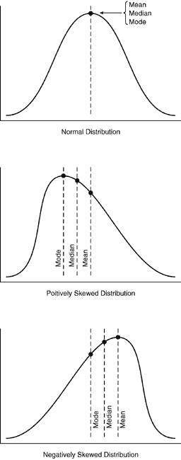
The median is defined as the middle value when the numbers are arranged in either ascending or descending order. When the distribution of data contains extreme values, the median often is a better indicator of the central tendency. The mode, on the other hand, is the value that occurs most often. All of these measures of central tendency indicate the overall shape of the distribution curve. When the mean, median, and mode all share the same value, then the resulting curve is said to be perfectly symmetric. Conversely, if the curve is skewed to the left or right, the mean, median, and mode values also are skewed to the left or right, respectively (Fig. 1).

Fig. 1. Measures of central tendency.

Back to Top
MEASURES OF DISPERSION
In addition to measures of central tendency, it is important to know how spread out the data set is. This is called variation or dispersion. Generally, the range, which is a measure of the difference between the largest and smallest value, provides a measure of dispersion within the data.
Back to Top
MEAN DEVIATION
Mean deviation is an important concept that defines the distance of the data points away from the median of the data points.
Back to Top
VARIANCE
Variance can be defined as the sum of the squared deviations of n measurements from the mean divided by n - 1, where n = the number of measurements, x = an individual observation, and xi = all of the subsequent data points.

Population-weighted variance:


σ2 = 1/N Σ(xi - μ)2

Sample-weighted variance:


s2 = 1/n - 1 Σ(xi - x)2

STANDARD DEVIATION

By taking the positive squared root of the variance, the standard deviation (SD) in the data set may be calculated as follows:


σ = √1/N Σ(xi - μ)2

Back to Top
PROPERTIES OF THE NORMAL DISTRIBUTION OR NORMAL CURVE
Using the assumption of a bell-shaped normally distributed curve, the following four important points may be noted:
  1. Within ±1 SD from the mean value for the data, 68% of the data is contained under the bell-shaped curve,
  2. Within ±2 SD from the mean valued for the data, 95% of the data is contained under the bell-shaped curve,
  3. Within ±3 SD from the mean value for the data, nearly 99.5% of all the data is contained under the bell-shaped curve.
  4. The area under the normal curve is equivalent to the probability of randomly selecting a value within that range and is equal to unity, or 1.
Back to Top
PARAMETRIC STATISTICS
Inferences, that is, possible conclusions, about the mean values based on a single sample can be calculated by first identifying both the null (Ho) and alternative (Ha) hypothesis. Only the null hypothesis actually is tested and refers to the fact that there is no evidence to support the hypothesis. If the null hypothesis can be rejected, then there is evidence for the alternative hypothesis (Ha). Typically, the null hypothesis is tested to a level of statistical significance in the range of p = .05, that is, the lowest range within which the null hypothesis can be rejected. Even at these levels of rejecting the null hypothesis, there is always the possibility that the null hypothesis was rejected when it actually was true. This is called a type I error. Using a possibility of p = .05 implies that the alpha (α) level is equal to .05, which means that there is a 1 in 20 chance that the data will show a significant difference when there is not one. Similarly, there is the slight chance that the null hypothesis will be incorrectly adopted when the alternative hypothesis is true. This possibility is known as a type II error or beta (β) error. In addition, it also is possible to derive the power of detecting the difference given a particular sample size. This is found using the formula (1 - β). In general, the larger the sample size, the smaller the standard error and the less the overlays between the two curves. Typically, a 10% or 20% (0.10 or 0.20) type II error is accepted.
Back to Top
CONFIDENCE INTERVALS
Thus far, the sample mean x has been estimated. This is known as a point estimate of the true value of the population mean μ. Typically, therefore, to account for the difference between the sample and population mean values, a confidence interval (CI) is constructed around the sample mean. By convention, statisticians use a 95% CI. This means that in all probability, 95% of the true mean of the population lies between the 95% CI determined from the sample. The 95% CI is found using the following formula:

  95% CI = sample mean ± 1.96 standard error
  or
  95% CI = x ± 1.96 standard error
  where: standard error = standard deviation = SD
  √sample size √n

Back to Top
TESTING HYPOTHESIS WITH THE “TEST” STATISTIC
The z-statistic is used when the SD is known.


z = x - μ/σx

When both μ and σ are known for a given population and the sample size is large (n > 30), it is possible to understand the pattern that the distribution of the sample mean will take. It is assumed that it has a normal distribution with a mean = μ and a standard error (σx) = σ/N. The critical region is defined as that region or area under the curve that includes values that will result in the rejection of the null hypothesis.

When the SD is unknown, a t-statistic is used. The t-statistic uses a ratio to assess the significance of the difference between the mean of two groups of data, such as observed or treatment group and a control. In general, the t-statistic is found using the following formula:

  x - μ/σx
  where: μ = population mean under the null hypothesis (Ho).

Last, with respect to the t-test, there is the concept of degrees of freedom (df). Thus, to calculate the number of degrees of freedom for problems using the t-distribution with a sample size n, 1 is subtracted from n (i.e., n - 1) to give the number of degrees of freedom (df) for a one-sample mean population.

Overall, both the z- and t-distributions and the calculation of their corresponding test statistic form the basis of calculating whether the two sets of data are significantly different from each other. This works for two sets of data, such as two treatment groups. However, among many sample means (e.g., from multiple treatment groups), the t-test is no longer valid. Rather, the more advanced statistical concepts of analysis of variance must be explored.

Back to Top
NONPARAMETRIC STATISTICS
Thus far, the methods described earlier have been based on the assumption that the data points have an underlying distribution that is normally distributed and all analytic techniques thus far have centered on describing the most important features, especially in terms of the central tendency and deviations. Nonparametric statistics, however, enables calculations and comparisons to be drawn between nominal and ordinal data, which primarily consist of examining the significance of the test between various categories.

Perhaps the most commonly used nonparametric test is the chi-square (ξ2) test, which measures the difference between the distribution of observed and expected values. The ξ2 test also can be used to examine the association between more than two variables, so long as the variables are nominal and the expected frequency in any one cell is greater than five. The basic formula for determining the Þgc2 statistic is as follows:


ξ2 (df) = Σ of all cells (observed - expected)2/expected

where: observed = the actual values; expected = values that would be anticipated given the calculation of the value for that cell based on the multiplication of the row and column values for that particular cell divided by the grand total for all rows and columns. The corresponding degrees of freedom (df) are found by subtracting one from each of the number of rows and columns and then multiplying them together, that is, df = (r - 1)(c - 1). If the calculated ξ2 value is greater than the given value for the ξ2 distribution with the exact same number of degrees of freedom, the null hypothesis must be rejected and it must be concluded that there is an association.

Other important nonparametric tests include the following: the binomial test, Fisher's exact test, the McNemar test, the Mann-Whitney U test, the Kolmogorov-Smirnov test, the sign test, and the Wilcoxon test. (The reader is advised to explore these in more detail by consulting the bibliography.)

Back to Top
INTERPRETING A DIAGNOSTIC TEST
In addition to being able to tell whether there is a statistically significant relationship between certain variables of interest, the ophthalmologist also is confronted by the unending barrage of instrumentation from which a clinical decision must be derived. Underlying the entire field of diagnostics are the basic concepts of sensitivity, specificity, negative and positive predictive values of a test, and the so-called receiver operating characteristics (ROC) curve.

The sensitivity of a test is the proportion of those with the disease (a + c) who also test positive (a) to the diagnostic test (a/[a + c]), whereas specificity is the proportion of those without the disease (b + d) who test negative (d) to the diagnostic test (d/[b + d]) (Table 3). Similarly, the predictive value of a positive test is given by (a + c)/(a + b), that is, all those with the disease (a + c) divided by all those testing positive to the disease (a + b). Conversely, the predictive value of a negative test is given by (b + d)/(c + d), that is, all those without the disease (b + d) divided by those testing positive to the disease (c + d) (see Table 3).


TABLE 3. Results of a Screening Test


TestDisease Present (D+)Disease Absent (D-)Total
Positive (T+ )aba + b
Negative (T)cdc + d
Totala + cb + da + b + c + d


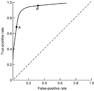
ROC curves originally were developed to measure the signal-to-noise ratio of early radio transmitters and have been adapted in the field of epidemiology to measure the true-positive values detected using the diagnostic test versus the false-negative values also picked up using the same diagnostic test. Thus, the ROC curve is a graph of the sensitivity (true-positive rate) to the false-positive rate. As shown in Figure 2, the closer the ROC curve is to the upper left-hand corner of the graph, the greater the accuracy of the test, since the true-positive rate is 1 and the false-positive rate is 0. Thus, as the values for a positive test become greater, the point on the curve corresponding to sensitivity and specificity (denoted by point A) decreases and moves to the left (i.e., lower sensitivity and higher specificity). Conversely, if fewer data are needed for a positive test, the point on the curve corresponding to sensitivity and specificity (denoted by point B) moves up and to the right (i.e., higher sensitivity and lower specificity). Last, the diagonal line drawn from the origin in Figure 2 represents a test with a positive or negative result purely by chance alone.

Fig. 2. Receiver operating characteristics curve.

Back to Top
AN OVERVIEW OF STUDY DESIGNS
There are many different types of study design to choose from when conducting an epidemiologic investigation. Often, the design that eventually is selected depends on a range of factors, such as how the data were stored, the completeness of the data files, and the feasibility of surveying the whole population versus selected samples of the population. Fortunately, only several epidemiologic study designs are commonly used.
Back to Top
CLINICAL TRIALS
Without a doubt, the clinical trial is the most rigorous of all epidemiologic study designs, requiring careful thought and adherence to the study protocol to determine a statistically significant effect between the treatment or intervention group and the control or placebo group. Moreover, patients who meet the enrollment criteria must be allocated to either one of the two groups in a random fashion to ensure that there is no allocation bias. This type of study design is sometimes called a double-blind (or double-masked) study, since neither the patient nor the evaluator of the treatment outcome knows whether the patient is on the new treatment or the control. A variation of the clinical trial design is the community-based trial, where an entire community is subject to a certain intervention and the health effects are observed in relation to a community that has been selected as the control group. A good ophthalmic example of this comes from examining the impact of the environmental modifications, such as the introduction of improved sanitation systems and vector control strategies, in the control and eradication of trachoma in developing countries.
Back to Top
OBSERVATIONAL STUDIES

PROSPECTIVE (COHORT OR LONGITUDINAL) STUDIES

Prospective studies start with a group or groups of patients free of the specific disease under investigation, yet each group is exposed to various known or unknown risk factors suspected or implicated in the development of the disease. The various cohorts then are followed longitudinally, that is, over time, to see whether certain cohorts develop the disease at different rates than other cohorts. Because there is no control group per se, all cohorts must be similarly constructed to minimize any potential sources of bias during the analysis period later on. In general, the more homogenous the cohorts the better, except with the exposure to possible risk factors under investigation, since any observed difference in disease severity will be more likely to result from variations in exposure rather than potential confounding variables. In general, prospective studies require a long follow-up period, often an individual's complete lifetime, and are thus costly to administer. Moreover, if the disease is rare, they require numerous enrollees. This said, prospective studies do carefully document the progression and onset of the disease in relation to other known health status indicators and risk factors.

RETROSPECTIVE (CASE-CONTROL) STUDIES

Retrospective studies are similar to prospective studies in that both a cohort of cases and a cohort of controls is identified, and then the strength of the relationship for a possible causal factor is determined using various means of determining measures of exposure to a given event or phenomenon often using personal exposure histories. As can be imagined, there is great room for recall bias on the part of the patients who may experience difficulty in fully remembering all of the necessary information to construct an epidemiologic association. Equally, because retrospective studies require knowledge of the patient's disease status before the intervention, it is difficult for the investigator to be absolutely convinced that the definition of a case actually matches the disease under investigation. A slight change in the definition of what is regarded as a case could drastically alter the interpretation of the data. Also, there is the concern that a control group has been properly and systematically identified, and it often is a problem to ensure that controls are equally matched for all clinically relevant variables. Despite these limitations, the retrospective study has the distinct advantage that it can be performed quickly at relatively low cost and is more amenable to studying rarer diseases, since cases can be collected from a much larger population. Case-control studies are particularly useful for obtaining pilot data to undertake more elaborate studies in the future.

CROSS-SECTIONAL STUDIES

Because the population is only sampled at one particular interval in time, that is, in a snapshot fashion, cross-sectional studies rely on the clear definition of cases (diseased) and controls (nondiseased). Cross-sectional studies are best suited to measure the prevalence of a particular disease or condition at a given point in time, such as the prevalence of visual acuity less than 3/60 (blindness according to the World Health Organization) in a given population at a point in time. The main limitation is that they provide only a one-time or snapshot view of the disease or condition, and this may not adequately reflect the true situation at that time or over a period of time.

CASE SERIES

A case series typically is a report of some clinically interesting finding or feature in a patient or group of patients. Because there are no control groups associated with the case series reports, the value of the case series study is lower than other studies involving an attempt to define a control group.

Back to Top
RATES
Epidemiology makes use of many different types of rates, all of which measure the change in some variable over time. Mortality and morbidity rates, for example, measure the number of deaths and severity of disease in a given population. Moreover, both mortality and morbidity rates can be cause specific, that is, attributable to a specific cause. In addition, one may tabulate both a crude rate, which is the rate of a given occurrence over an entire population (e.g., the number of cataract operation per 100,000 of the population), and an age-specific rate, such as the age-specific rate of cataract surgery among those 65 years or older. Incidence rates always are expressed in units of time, whereas prevalence rates are for a given time. The incidence rate is the number of new cases of a given disease occurring over a defined period of time divided by the total number of persons at risk since the start of the same time period. The prevalence rate of a disease is defined as the number of persons with a given disease at any one time divided by the total number of persons in the population at risk at that time.
Back to Top
RELATIVE RISK RATIOS
In epidemiology, it often is useful to know the ratio of the presence of a given disease in people exposed to a suspected cause or risk factor to those who were not exposed to the risk factor. Relative risk provides such a measure and must be calculated from a cohort study or a clinical trial in which a group of patients with exposure to the risk factor and a group of patients without this exposure are followed over time to determine which patients develop the finding of interest. If the relative risk is less than 1, it is considered to be protective of developing the outcome of interest, whereas if the relative risk is greater than 1, it is regarded as promoting the outcome of interest. Table 4 presents an easy way to determine the relative risk in a prospective study.


TABLE 4. Calculation of Relative Risk and Odds Ratios


Risk FactorDiseasedNondiseasedTotal
Presentaba + b (Persons With Risk Factors)
Absentcdc + d (Persons Without Risk Factors)
Totala + cb + d 
The relative risk is equal to the incidence of disease among those with the risk factor divided by the incidence of disease among those without the risk factor. Mathematically, this can be expressed as:
 

The odds ratio can be calculated according to the following mathematical formula:
 

which simplifies down to the cross-product ratio:


Back to Top
ODDS RATIO
Often, the relative risk ratio cannot be easily calculated. This is especially true when only case-control data are available. Under these circumstances, the incidence rates must be estimated using the odds ratio. This refers to the odds that a given patient was exposed to a given risk factor divided by the odds that a given person from the control group also was exposed. The odds ratio sometimes is called the cross-product ratio (see Table 4).
Back to Top
SAMPLE SIZE
Perhaps one of the more important aspects in conducting any epidemiologic study is to determine the sample size required to detect a statistically significant difference between the control and intervention groups. If too few patients are enrolled in the study, then it will be difficult to know if the observed difference is statistically significant or whether it occurred purely by chance. Conversely, if too many individuals are enrolled in the study, precious resources may be wasted or it may take too long. Overall, there are two main points to consider when calculating the required sample size, namely, the effect size and the power of the study.

The effect size refers to the difference between both the control and intervention groups, which need to be detected. Thus, to calculate the necessary sample size, one must know the smallest difference between the two treatments that would miss detection, or not be detected at all. Overall, the effect size may be thought of as the degree to which the phenomenon is present in the population; it measures the degree of difference between the intervention and control group.

Power refers to the probability of detecting a real effect if it is present. Recall that to calculate the power, the following equation must be used, namely, 1 - β. In general, power values of .8 (80%) or higher are selected when conducting a clinical trial. Thus, with a power of 0.8 (80%), the probability of a type II error is 0.2 (20%). Table 5 presents a range of sample size calculations to attain desired power and effect sizes.


TABLE 5. Sample Size Calculations


Significance Level = .05AssumptionsEffect SizeDesired PowerSample Size
 Control group response rate on order ofDetect increased in treatment group on the order of:Given a probability ofNo. needed in each group
1-tailed30%40%.8280
2-tailed30%40%.8356
(Adapted from Wassertheil-Smoller S: Biostatistics and Epidemiology: A Primer for Health Professionals, p 143. New York: Springer-Verlag, 1995.)


Back to Top
BIBLIOGRAPHY

ANALYSIS OF VARIANCE

1. Daly LE, Bourke GJ, McGilvaray J: Interpretation and Uses of Medical Statistics, pp 139–156, 245–248. 4th ed. Oxford, UK: Blackwell Scientific, 1991

2. Armitage P, Berry G: Statistical Methods in Medical Research, pp 207–228. 3rd ed. Oxford, UK: Blackwell Scientific, 1994

Back to Top

NONPARAMETRIC STATISTICS

1a. Bland M: An Introduction to Medical Statistics, pp 216–218. Oxford, Oxford Medical Publications, 1993

1b. Campbell MJ, Machin D: Medical Statistics: A Comprehensive Approach, pp 83, 84, 150–152. 2nd ed. Chichester, UK: John Wiley & Sons, 1993

Back to Top