Chapter 30
Geometrical Optics
EDMOND H. THALL
Main Menu   Table Of Contents

Search

BASIC DEFINITIONS
ADDITIONAL DEFINITIONS
PROPERTIES OF IDEAL LENSES
INFINITE CONJUGATES AND FOCAL PLANES
GRAPHICALLY LOCATING THE IMAGE
LOCATING IMAGES BY VERGENCE
VIRTUAL IMAGES AND VIRTUAL OBJECTS
REFERENCES
FERMAT'S PRINCIPLE, REFRACTION, AND REFLECTION
THE SPHERICAL REFRACTING SURFACE
THE PARAXIAL POWER OF A SPHERICAL SURFACE
THE THIN LENS APPROXIMATION
LENS SHAPE AND FABRICATION
THICK LENSES
REDUCED VERGENCE
AXIAL MAGNIFICATION
AFOCAL SYSTEMS
THE NONSTIGMATIC IMAGE
DIFFRACTION
ABERRATIONS
IMAGE QUALITY
APERTURES
CYLINDRICAL LENSES
PRISMS
CLINICAL EXAMPLES
ACKNOWLEDGMENTS
SINGLE, POSITIVE, SPHERICAL REFRACTING SURFACE
SINGLE, NEGATIVE, SPHERICAL REFRACTING SURFACE
POSITIVE THIN LENS, SAME MEDIUM ON BOTH SIDES OF THE LENS
POSITIVE THIN LENS, DIFFERENT MEDIUM ON EACH SIDE
NEGATIVE THIN LENS, SAME MEDIUM ON EACH SIDE
NEGATIVE THIN LENS, DIFFERENT MEDIUM ON EACH SIDE
POSITIVE THICK LENS IN AIR
NEGATIVE THICK LENS IN AIR
POSITIVE THICK LENS IN WATER
NEGATIVE THICK LENS IN WATER
CALCULATING THE CRITICAL ANGLE FOR TOTAL INTERNAL REFLECTION
VECTORS
CALCULATING SURGICALLY INDUCED CHANGE IN CORNEAL POWER
REFERENCES

The discipline of geometrical optics deals with image formation by optical instruments. Physical optics (see elsewhere in these volumes) deals with the nature of light itself (e.g., electromagnetic waves and photons). In contrast, geometrical optics deals with the various pathways light travels as it moves from an object, through an optical system, and, ultimately, arrives at the image. Interestingly, image properties depend primarily on the routes light travels rather than on the nature of light per se.

The refracting lane is an ideal laboratory for demonstrating the principles of geometrical optics. Light a candle and extinguish all other illumination. Stand a few meters from the candle and hold a + 4.00 D spherical convex trial lens about 25 cm in front of a sheet of plain white paper and observe the flame's inverted image. In the same way, the ocular media produce images on the retina. The clinician should understand the factors that influence the image's characteristics (e.g., size, location, and so forth), the effects of pathology on the image, and how to use this information both diagnostically and therapeutically.

This chapter presents the theory of geometrical optics and then gives examples illustrating the application of theory to clinical practice. The treatment is largely qualitative. Mathematical details are in the Appendix.

Back to Top
BASIC DEFINITIONS
The word lens may refer to a single piece of glass (or other material) or to a combination of individual lenses assembled to function as a unit. Element refers specifically to an individual lens. Figure 1 shows a high-quality camera lens consisting of six elements.

Fig. 1. A common photographic lens consisting of six individual elements.

A rotationally symmetric optical system has an axis of symmetry called the optical axis (Figs. 1 and 2). Rotating the system about the axis does not alter the imaging characteristics. Rotationally asymmetric systems do not have an axis. Look through a -1.00 D spherical trial lens. Rotate the lens and notice that the scene does not change. Replace the spherical lens with a prism or cylinder and observe how the scene changes as the lens rotates. Thus, cylinders and prisms are not rotationally symmetric.

Fig. 2. Most optical systems consist of several lenses symmetrically arranged along a common axis.

A vertex is any intersection of the axis with a lens surface (Fig. 3). At the vertex, the axis is normal (i.e., perpendicular) to the lens surface.

Fig. 3. The vertices are the intersections of the lens surfaces with the axis. The axis is perpendicular to the lens surfaces at the vertices.

OBJECTS

An object may be luminous or nonluminous. A luminous object or source produces light and is visible in otherwise total darkness. Every point on a luminous object radiates light in all directions (Fig. 4). Nonluminous objects do not produce light and are visible only when illuminated by a source. When light strikes a point on a nonluminous object, it is diffusely reflected or scattered in all directions (Fig. 5).

Fig. 4. Every point of a luminous object (e.g., candle flame) radiates light in all directions.

Fig. 5. Nonluminous objects scatter light in all directions.

Diffuse reflection should not be confused with specular reflection. In specular reflection, light symmetrically rebounds in a single direction instead of scattering in many directions (Fig. 6). From the standpoint of geometrical optics, the most important characteristic of an object, whether luminous or nonluminous, is that every point of the object radiates light in all directions. Surfaces that reflect specularly are mirrors, not objects.

Fig. 6. In specular reflection, the incident light symmetrically rebounds from the surface.

A point source (Fig. 7) occupies no volume (i.e., a point in the mathematical sense) and radiates light in all directions. Point sources do not exist, but conceptually, objects are simply a collection of point sources. Every object point is a point source radiating in all directions. Point sources simplify the analysis of optical systems by making it possible to deal with one object point at a time.

Fig. 7. A point source radiates light in all directions.

THE STIGMATIC IMAGE

Each point on a screen (e.g., piece of paper) placed near an object receives light from many object points (Fig. 8), and no image appears. An appropriate lens placed between screen and object redirects light so that each point on the screen receives light from a single object point (Fig. 9), thereby producing an image. Without the lens, light from a single object point distributes over the entire screen, mixing with light from every other object point. With the lens, however, light from a single object point falls on a single screen point and does not mix with light from any other object point.

Fig. 8. Each point on the screen receives light from multiple object points. No image is produced.

Fig. 9. The lens redirects light so that each point on the screen receives light from only one object point. An image is produced.

The one-to-one correspondence between object and image points is the essential feature of the stigmatic image. The word stigmatic derives from the Greek “stigma,” meaning stylus or point, and emphasizes the point-to-point nature of the stigmatic image.

Imaging is a two-step process. In the first step, an object distributes light in all directions. This is an important step. If an object radiates light in only one direction, then it will be visible from only one vantage point (Fig. 10). Scattering light makes objects visible from many directions simultaneously (Fig. 11). Although beneficial, scattering necessitates a second step, the redirection of light by an optical system to produce an image.

Fig. 10. If the object scattered light in only one direction, it would be visible to only one observer.

Fig. 11. Objects scatter in many directions and thus are visible to several observers simultaneously.

THE IDEAL IMAGE

Besides stigmatism, there are other desirable image properties. The image of a flat object that is normal to the axis should, likewise, be flat and normal to the axis. Some lenses produce stigmatic, but curved, images. The technical term for this is field curvature. Photographic film is usually flat. A photograph of a curved image taken with flat film is out of focus at the edges (Figs. 12 and 13). Of course, the retina is curved, but the macula is flat. Only the macula is capable of high acuity, so field curvature is undesirable in the eye.

Fig. 12. Non-ideal optical systems may image planes perpendicular to the axis as curved surfaces. If this is a camera using a flat piece of film, the photograph will be blurry at the edges.

Fig. 13. Photograph was taken using a + 4.00 D trial lens. The image is out of focus at the edges because of field curvature.

Figure 14 shows a photograph of an Amsler grid. The image is stigmatic and flat, but distorted. The image does not preserve the spatial relationship of the object points. For that matter, enlarged, reduced, or inverted images do not preserve the spatial relationship of the object points either. However, an enlarged image differs from the original object by only a scale factor. Distortion is a greater disruption of the image. No simple change in scale can make a distorted image resemble the object.

Fig. 14. Photograph of an Amsler grid. Straight lines appear to curve toward the center because of the pincushion distortion. The effect is most pronounced at the edges.

Field curvature and distortion are not always undesirable. Photographers use distortion for aesthetic effects. Panoramic cameras have field curvature but use curved film to compensate. Nevertheless, geometrical optics defines the ideal image as stigmatic and free of field curvature or distortion. The ideal image may be enlarged, reduced, or inverted with respect to the object.

RAYS

A ray is an abstract representation of a light path. An arrow indicates the propagation direction. Rays represent paths, not the light moving along those paths. A ray gives no indication of the physical characteristics (e.g., intensity, wavelength, and so forth) of the light traveling along the ray.

It may seem somewhat pedantic, but lenses bend light, not rays. When a ray strikes the surface of a lens or mirror, it does not deviate. The light moving along the ray changes direction and begins to move along a new ray. Rays continue straight through the surface of a mirror or a lens, but the light does not (Fig. 15). Rays extend infinitely in both directions. Light travels over only a segment of the ray. The distinction between a ray and the light moving along a ray becomes important later when dealing with pupils and virtual images. For clarity, illustrations usually show only the portion of a ray over which light travels, but rays are straight and infinite in extent.

Fig. 15. Technically, a ray never deviates. The ray extends as a straight line to infinity. Lenses (or mirrors) do not change the ray's direction. At the lens, the light traveling along the ray changes direction. The light stops moving along the object ray and begins moving along the image ray.

It must be noted that it is common practice and more economical to use statements such as “the lens bends the ray” instead of “the lens bends light traveling along the ray.” Of course, the implication is that the light bends, not the ray.

Any ray that intersects the object point is an object ray. Similarly, image rays intersect the image point. Object rays represent light before it has entered the optical system, and image rays represent light after it emerges from the system. Every object ray entering an optical system gives rise to a unique image ray. Thus, every object ray is associated with a unique image ray, and vice versa.

Back to Top
ADDITIONAL DEFINITIONS
Before proceeding, some additional definitions will be helpful. An ideal lens is a rotationally symmetric optical system that produces an ideal image of any object. At this point the imaging properties of the lens are the main concern, and there is no need to worry about how many elements are in the lens or any other aspects of its construction. Consequently, ideal lenses are illustrated as “black boxes” (Fig. 16).

Fig. 16. Planes perpendicular to the optical axis are imaged (top), ideally, as planes perpendicular to the axis. Planes (bottom) tilted with respect to the axis are imaged, ideally, as planes tilted with respect to the axis.

Objects are usually three-dimensional, but it is easier to describe optical properties using flat objects confined to planes. An object plane is normal to the axis and contains an object (see Fig. 16). Every point in an object plane is a potential object point or point source. Image planes are normal to the axis, and every point in the image plane is a potential image point.

Conjugate refers, in a rather general way, to the object-image relationship. Let O and O' be, respectively, an object point and its image. O is conjugate to O'. Similarly, O' is conjugate to O.

Collectively, O and O' constitute a pair of conjugate points.

Transverse magnification is the ratio of image height to object height. Two aspects of magnification are confusing. In common parlance, magnification implies enlargement, but in optics, magnification applies to any image whether larger or smaller than the object. Images are scale models of the object, and magnification is the scale factor. Magnification also indicates the image's orientation with respect to the object. A negative magnification indicates an inverted image. For example, a magnification of -2 means the image is inverted and twice the size of the object. A magnification of 0.5 indicates that the image is upright and half the size of the original.

Transverse magnification applies to linear dimension. Thus, a 1-inch-wide, 2-inch-high object magnified by a factor of two gives a 2-inch-wide, 4-inch-high image. Both the height and width change by a factor of two, increasing the image's area by a factor of four.

Back to Top
PROPERTIES OF IDEAL LENSES
The ideal lens produces a one-to-one correspondence between object points and image points. Consequently, no two object points share the same image point. Thus, necessarily, the image of every object point has a different location in space.

Consider two points P and Q imaged by an ideal lens to conjugates P' and Q', respectively (Fig. 17). One particular ray happens to go through both object points P and Q. This object ray will produce an image ray that must pass through both image points P' and Q'. Light originating from P travels along the ray and must reach P'. Similarly, light originating from Q travels along this ray and must reach Q'. So, the image ray associated with this particular object ray must go through both image points.

Fig. 17. P' and Q' are the images of P and Q, respectively (top). An object ray that intersects both object points P and Q must produce an image ray that intersects P' and Q'. Extending the reasoning, every point on the object ray has an image somewhere on the image ray (bottom).

This reasoning extends to every point on an object ray. Every point on an object ray has a unique image point, and the image ray associated with the object ray passes through all of these image points. The object ray and its associate image ray are conjugate. To summarize, light moving along an object ray enters an optical system, deviates, and emerges, traveling along an image ray. Every point on the object ray must have an image somewhere on the image ray.

From a clinical viewpoint, the most important property of ideal lenses deals with object and image planes. Associated with every object plane is a unique image plane. Every point in the object plane has an image somewhere in the associated image plane (i.e., the object and image planes are conjugate). No two object planes share the same image plane; every object plane has an image plane in a different location (Fig. 18). This property seems inconsistent with daily experience. To be seen clearly, the image must be on the retina. According to this property, only one object can have an image plane on the retina at any one time; despite this fact, everything in a scene seems to be in focus simultaneously.

Fig. 18. Every object plane has a different image plane. A map can be constructed for an ideal imaging system showing the image locations associated with various object locations. Note the changes in magnification. Different (ideal) imaging systems give different maps. (m, magnification)

How can the properties of imaging systems be reconciled with common experience? First, the impression that all objects in a scene are in focus simultaneously is not correct. Carefully observe a scene with both near (about 18 inches) and distant (about 6 feet) objects. Notice that when the near objects are clear, the far objects are blurry, and vice versa. We have a mistaken notion that everything is in focus simultaneously because we pay attention only to part of a scene at any one time. As we shift our attention, the eye keeps various objects in focus by varying accommodation. Nevertheless, many objects are simultaneously in focus despite being various distances from the observer. This is due to depth-of-focus, a property of optical systems discussed later.

In any case, image position changes as object position changes. Magnification also changes with object position. For example, there is only one object position that gives an image with a magnification of 2. Any magnification is attainable with an ideal lens, but only if the object is in the correct location. A sort of map can be constructed that identifies the image plane location for various object planes (see Fig. 18). The map can also indicate magnification.

Image position also depends on lens power. Repeat the candle and lens demonstration using different power lenses while maintaining a constant distance between candle and lens. Again, the image position varies with lens power. The maps depicted in Figure 18 vary for every different ideal lens.

An important aspect of geometrical optics is the ability to predict image position and size theoretically (given the object position and lens power) without going to the trouble of doing the experiment.

Back to Top
INFINITE CONJUGATES AND FOCAL PLANES
As the distance between an object point and lens increases, the object rays tend to become parallel (Fig. 19). It takes a little imagination, but rays from an infinitely distant object point are parallel. When the infinitely distant object point is on the optical axis, the object rays will be parallel to each other and parallel to the axis. If the distant object point is not on the axis, the object rays are still parallel to each other, but not parallel to the axis (Fig. 20).

Fig. 19. The amount of divergence of the light is inversely proportional to the distance from the source. If the distance is expressed in meters, the vergence is in units of diopters: 1\Distance in Meters = Diopters. Since A < B, 1\A > 1B . (The light at distance A has more vergence than that at B.) Since C = ∞ , 1\∞ = 0. For example, if we go far enough, the vergence is zero.

Fig. 20. Rays from an infinitely distant object point on the axis yield rays parallel to the axis (top). Rays from an infinitely distant object off axis yield rays parallel to each other but not parallel to the axis (bottom).

When the rays emerging from a lens are strongly convergent, the image is close to the lens. The less divergent the rays, the farther the image from the lens. If the image rays are parallel, the image point is at infinity. Image rays parallel to each other and also parallel to the axis give an infinitely distant image point on the axis. Image rays parallel to each other but not parallel to the axis give infinitely distant image points off-axis.

Objects that are not infinitely distant but far away give rays that are nearly parallel. Objects 20 feet (6 m) or more distant give rays so close to parallel that, for clinical purposes, they may be considered at infinity.

Object rays parallel to each other and to the axis produce image rays that converge at the secondary focal point. Because the object rays arose from an infinitely distant object point, the secondary focal point is the image of an on-axis object point at infinity. The secondary focal plane is normal to the axis through the secondary focal point. Off-axis points at infinity image at various points on the secondary focal plane (Fig. 21).

Fig. 21. Rays from an on-axis object point at infinity image at the focal point. Rays from an off-axis object point at infinity image on the focal plane.

An object point at the primary focal point produces image rays that are parallel to each other and the axis (Fig. 22). Thus, the primary focal point's image is on-axis at infinity. The primary focal plane is normal to the axis through the primary focal point. Object points on the primary focal plane give image rays that are parallel to each other but not necessarily parallel to the axis (see Fig. 22).

Fig. 22. Object rays from the secondary focal point emerge as image rays parallel to each other and to the axis (top). Object rays from a point on the secondary focal plane emerge as image rays parallel to each other but not necessarily to the axis (bottom).

Back to Top
GRAPHICALLY LOCATING THE IMAGE
This section describes a means of locating the image using a graphical technique called ray sketching. This method is easy to use but requires a rather detailed explanation.

Image location partially depends on the properties of the lens. Thus, it is impossible to locate an image by any method without some specific information about the lens. In ray sketching, the cardinal points contain the lens information.

Consider an ideal lens. For every object plane there is a unique conjugate image plane and a unique magnification. There is one pair of conjugate planes that yields a magnification exactly equal to 1 (Fig. 23). In other words, an object located at P in Figure 23 has an image in plane P', and the image has the same size and orientation as the original object. This specific pair of conjugate planes is called the principal planes or planes of unit magnification. The object plane P is the primary principal plane, and the image plane P' is the secondary principal plane.* The points of intersection of planes P and P' with the optical axis are, respectively, the primary and secondary principal points.

Fig. 23. The principal planes are the planes of unit magnification (m). Thus, an object placed in the primary principal plane will be imaged upright and actual size at the secondary principal plane.


Many textbooks use the terms front and back instead of primary and secondary. However, in some lenses the “front” principal plane can be behind the “back” principal plane. To avoid confusion, this text uses the directionally neutral terms primary and secondary.

The nodal points are another pair of useful landmarks located on the axis. An object ray passing through the primary nodal point is conjugate to an image ray passing through the secondary nodal point, and both rays make the same angle with the optical axis (Fig. 24). There are no nodal planes associated with the nodal points.

Fig. 24. An object ray passing through the primary nodal point (N) emerges at the same angle from the secondary nodal point (N'). The ray is displaced but unchanged in direction.

Collectively, the principal, focal, and nodal points constitute the cardinal points of the optical system. All the information about the lens and its imaging properties is contained in the position of these points on the axis. Fundamentally, the only difference between two ideal imaging systems is the location of their cardinal points.

RAY SKETCHING

The ray sketching method for locating an image can now be described. Starting with an ideal optical system, the task is to determine image location and size for a given object (Fig. 25).

Fig. 25. An optical system showing the location of the cardinal points and an object. Where is the image formed and what is the magnification?

STEP 1.

Ignore the presence of the lenses because the locations of the cardinal points completely determine the properties of an ideal system. If necessary, redraw the object and optical system to scale using just the optical axis and cardinal points. Draw the principal planes through the principal points and normal to the axis (Fig. 26).

Fig. 26. Ray sketching. Step 1: Redraw the system to scale omitting the lenses. Draw the principal planes normal to the axis and through the principal points.

STEP 2.

Pick some point on the object but not on the optical axis. Rays emanate from this point in all directions. In particular, one of these rays will be parallel to the optical axis. Draw the ray parallel to the axis from the object point to the primary principal plane (Fig. 27). Conceptually, this ray extends backward to infinity; in principle, this ray goes through the axial object point at infinity.

Fig. 27. Step 2: Select an object point not on the optical axis and draw the ray parallel to the axis. Designate the point where this ray meets the primary principal plane as M. The image of M is located on the secondary principal plane at M'.

STEP 3.

The object ray drawn in step 2 goes through two important object points: 1) the axial object point at infinity and 2) a point on the primary principal plane (point M). The image ray must go through the images of these two object points. The image of M is M'. M' is a point on the secondary principal plane at the same height above the axis as point M because the principal planes are conjugate with a magnification of 1. Thus, the image ray must go through M' and the secondary focal point. The image ray is drawn through these two points (Fig. 28).

Fig. 28. Step 3: Draw the image ray through points M' and F' and extend it.

STEP 4.

Many other rays emanate from the object point, including one that goes through the primary image point F. Draw this ray and extend it to the principal plane (Fig. 29).

Fig. 29. Step 4: Draw another ray from the object point through the primary focal point F and extend it to the primary principal plane. Designate Q as the point of intersection with the primary principal plane.

STEP 5.

The ray drawn in step 5 must be conjugate to an image ray parallel to the axis (because the object ray goes through the primary focal point). The image ray must also pass through Q', the image of Q. Draw the second image ray through Q' and parallel to the axis (Fig. 30).

Fig. 30. Step 5: Draw the image of the ray drawn in step 4. The image ray is parallel to the axis and through the point Q'. The two image rays intersect at the image point.

STEP 6.

All the rays from the object point must intersect at the image point, so the two rays just drawn must also intersect at the image point. The intersection of the two image rays locates one image point. The rest of the image is drawn normal to the axis (Fig. 31).

Fig. 31. Step 6: Draw the rest of the image perpendicular to the axis and through the image point. Because the drawing is to scale, the magnification can be found by measuring the object and image heights and taking the ratio. The magnification for this example is m = -1.6. The negative sign indicates the inverted image.

STEP 7.

Only two rays are necessary to locate the image, but it may help to draw a third ray from the object point to the primary nodal point N (Fig. 32).

Fig. 32. Step 7: As a check, draw a third ray from the object point to N.

STEP 8.

The image ray conjugate to the object ray drawn in step 7 goes through the secondary nodal point and is parallel to the object ray (Fig. 33). This ray should intersect the other two at the image point.

Fig. 33. Step 8: This ray emerges from N' without a change in angle. If the drawing is correct, then this ray should intersect the other two image rays at a common point.

With a little practice, ray sketching becomes second nature. However, an understanding of why ray sketching works is more important than facility with the technique. The value of ray sketching is more pedagogical than practical. Ray sketching is not used on a daily basis, but it is helpful when one is confronted with a new or unfamiliar optical system.

To summarize, rays emerge from an object point in all directions, and there is no easy way to determine the image rays associated with most of these object rays. However, for three special object rays, the conjugate image rays can be determined with the aid of the cardinal points. These three special object rays are: 1) the ray parallel to the axis, 2) the ray through the primary focal point F, and 3) the ray through the primary nodal point N. The intersection of the image rays conjugate to these object rays locates the image.

It is important to realize that ray sketching does not give the actual path of a ray within the lens itself. Ray sketching gives only the final image ray associated with a particular object ray. Figure 34 compares a ray sketch with the actual path of light traversing a thick lens. Although ray sketching does not give the true light path, the ray that finally emerges does coincide with the image ray predicted by ray sketching.

Fig. 34. Comparison of a ray sketch with the actual path a ray follows through a lens. The path is not the same as the ray sketch, but the final image rays do coincide.

In other words, ray sketching gives the correct final answer, but the intermediate details are wrong. With use of a different technique called ray tracing, it is possible to determine the exact path light follows. Ray tracing requires a detailed description of the optical system (not just the cardinal points) and considerable calculation. The strength of ray sketching is that it skips all the intermediate details and gives the correct result without calculation. The gain in simplicity comes at the expense of detailed information about the light path within the lens system itself.

Back to Top
LOCATING IMAGES BY VERGENCE
In the examples described so far, light diverges from the object point and converges to the image point. Vergence is a quantitative measure of light's degree of convergence or divergence. As noted previously, when distance from an object point increases, divergence decreases (see Fig. 19). Similarly, as distance from the image point increases, convergence decreases. Thus, vergence is inversely proportional to distance from an object or image point. By convention, divergent light has a negative vergence, and convergent light has a positive vergence.

Vergence is a property of a ray, and every point on a ray has a different vergence. To give a concrete example, consider an object point 25 cm away from the primary principal plane of an ideal lens and 5 cm in front of the primary focal plane (Fig. 35). When rays from the object point cross the primary focal plane, they have a vergence of -20.00 D. The vergence is negative because the light is divergent. The number 20.00 is the reciprocal of the distance in meters between the object point and focal plane (5 cm = 0.05 m, 1/0.05 = 20). The uppercase “D” is the standard abbreviation for diopter. The diopter is the standard unit of vergence used clinically. When the light reaches the primary principal plane, the vergence is -4.00 D. Again, the vergence is negative because the light is divergent. The number 4 is the reciprocal of the distance between the object point and principal plane (0.25 m).

Fig. 35. Every point on a ray has a different vergence. The vergence of any particular point is inversely proportional to the distance from (or to) the object (or image) point.

Upon emerging from the lens, the light's vergence has changed. An ideal lens is simply a vergence changer. The power of the lens specifies the amount of vergence change the lens produces. The lens in Figure 35 has a power of + 5.00 D. Thus, light with a vergence of -4.00 D has a vergence of + 1.00 D (= -4.00 D + 5.00 D) at the secondary principal plane. The image is 1 m behind the secondary principal plane. The distance is found by taking the reciprocal of the vergence.

To give a second example, if the object point in Figure 35 were 25 cm from the primary principal plane, then light (at the primary principal plane) would have a vergence of -4.00 D. The lens changes the vergence by + 5.00 D, giving light at the secondary principal plane a vergence of + 1.00 D. The image is 100 cm behind the secondary principal plane. The Appendix gives additional examples.

Vergence is the reciprocal of distance. Units of length, or distance, include inches, meters, centimeters, and so forth. Therefore, the units of vergence are reciprocal inches (in)-1), reciprocal meters (m)-1), reciprocal centimeters (cm)-1), and so forth. Vergence is expressible in any of these inverse units. However, lens power and vergence add only when both are in the same units. To avoid confusion, it is universal clinical practice to use units of inverse meters for both vergence and lens power. The unit of diopter was created as a matter of convenience. By definition, one diopter equals one inverse meter.

It is conventional practice to round vergence to two decimal places, and the sign, whether positive or negative, should always be written. In most mathematical work, plus signs are redundant and not written, but the most common mistake in vergence calculations is inadvertently dropping a minus sign. Always writing the sign helps to prevent this.

Transverse magnification can be calculated by use of vergence. The ratio of object vergence to image vergence gives the transverse magnification. In the first example of this section, the transverse magnification is -4.00 (= -4.00 D/+ 1.00 D). In the second example, magnification is -2/3 (= -2.00 D/+ 3.00 D).

Finally, note that parallel light rays neither converge nor diverge, and thus have a vergence of zero diopters. By convention, light from objects or images more than 20 feet away is so close to parallel that it is assigned a vergence of zero.

Back to Top
VIRTUAL IMAGES AND VIRTUAL OBJECTS
Where is the image of an object 12.5 cm in front of a + 3.00 D lens? The object vergence is -8.00 D (at the lens), so the image vergence is -5.00 D. The negative vergence means that the image rays emerging from the lens are still divergent. The ray sketch is shown in Figure 36. Unlike previous examples, the lens does not have enough power to convert the divergent object rays into convergent image rays. Granted, the image rays are less divergent than the object rays (by three diopters in this case), but the image rays remain divergent. There is no real image, and this can be verified by use of a candle and trial lens.

Fig. 36. The object point is so close to the lens that the image rays emerging from the lens are divergent.

Suppose a + 6.00 D lens is placed 5 cm behind the original + 3.00 D lens. The divergent light emerging from the first lens reaches the second lens, which does have enough power to converge light and form a real image. What is the location of the image formed by the second lens?

To answer this question, it is necessary to know the vergence of light incident on the second lens. Light has a vergence of -5.00 D when it emerges from the first lens, but the vergence changes as the light travels from the first lens to the second lens. The change in vergence produced simply by light moving from one place to another within the same medium is the vergence change on transfer. Because of the vergence change on transfer, it is necessary to determine the vergence of the light incident on the second lens.

Vergence is always related to the distance between an object or image point and some point of interest on the ray (such as the point where the ray meets the lens). Thus, to determine the vergence of the light incident on the second lens, the image rays emerging from the first lens must be associated with some image point. The image point is found by extending the divergent image rays backward until they meet at a common point (Fig. 37). In this case, the image point is 20 cm in front of the first lens (found by taking the reciprocal of the vergence).

Fig. 37. The first lens creates a virtual image that becomes the object point for the second lens, which has enough power to converge the rays and form a real image.

No light goes through this virtual image point. Light does not travel over the part of the image rays extended backward. The virtual image point is a mathematical construct; if a piece of paper is placed 20 cm in front of the first lens, no image will be observed. This mathematical construct is called virtual because it does not represent a real image. It is called an image because it is associated with the image rays emerging from the first lens.

The virtual image is 25 cm in front of the second lens. Thus, light incident on the second lens has a vergence of -4.00 D. Light emerging from the second lens has a vergence of + 2.00 D, giving an image 50 cm behind the second lens.

Next, consider an object far away from a + 2.00 D lens. The lens forms an image 50 cm behind itself. Where is the image if a + 6.00 D lens is placed 25 cm behind the first lens (Fig. 38) Again, the vergence of the light incident on the second lens is the key issue. Light incident on a lens from a real object is always divergent. However, in this case, the light incident on the second lens is convergent. The convergent light is associated with an object point 50 cm behind the lens, but real objects are always in front of a lens. This example represents a virtual object. The virtual object is 25 cm behind the second lens, giving the incident light a vergence of + 4.00 D. Rays emerging from the second lens have a vergence of + 10.00 D, giving an image 10 cm behind the second lens.

Fig. 38. The first lens creates a virtual image that becomes the object for the second lens.

It is often incorrectly stated that real images are always inverted and virtual images are erect. There is no inherent relationship between an image's orientation and its status as real or virtual. An image is real if the image rays are convergent, and virtual if the image rays are divergent. An object is real if the object rays are divergent, and virtual if the object rays are convergent.

An important difference between the examples in this section and those of previous sections is that these cases involve more than one element. Virtual images and objects are primarily mathematical tools (but very useful ones) for dealing with multiple lenses.

Back to Top
REFRACTIVE INDEX
A medium is anything that light can travel through, such as glass, liquids, air, a vacuum, and even some metals. The speed of light varies in each medium. Light travels fastest in a vacuum and slower in any material medium.

Rather than deal directly with light's speed in a medium, it is usually more convenient to use refractive index. The refractive index of a medium is the ratio of light's speed in the vacuum to its speed in the medium. For example, the refractive index of spectacle crown glass is 1.523, indicating that light's speed in glass is about two-thirds its speed in a vacuum. Refractive index is always a number greater than or equal to 1. It is routine practice to use the lowercase letter “n” to indicate refractive index in formulas and equations.

Refractive index varies with wavelength. In general, the shorter the wavelength, the higher the refractive index. For instance, in spectacle crown glass, light of wavelength 656 nm (corresponding to red) has an index of 1.520, whereas light of wavelength 480 nm (corresponding to blue) has an index of 1.531. Dispersion is the variation of refractive index with wavelength. In the crown glass example, the dispersion is 0.011 (= 1.531 - 1.520). Each medium exhibits a different amount of dispersion, and not all media are dispersive. All wavelengths travel the same speed in a vacuum. The dispersion of air is so small that it can be ignored.

Refractive index is quite sensitive to chemical composition. It is easy to measure the refractive index difference between distilled water and physiologic saline. In the past, glycosuria was diagnosed by measuring urine refractive index. Manufacturers alter the optical properties of glass by adding small amounts of rare earth elements such as barium. Over 200 different types of optical glass with different indices (and dispersions) are commercially available.

Environmental factors such as temperature and atmospheric pressure can also influence refractive index, but the effects are usually small enough to be ignored. A notable exception is the index of silicone (20°C), which is strongly temperature dependent. Manufacturers should measure the power of silicone intraocular lenses at (or adjusted for) eye temperature (35°C) rather than at room temperature, or a clinically significant error in power may occur. Humidity can affect the refractive index of soft contact lenses by altering the water content.

Back to Top
FERMAT'S PRINCIPLE, REFRACTION, AND REFLECTION
Optical systems produce images by redirecting light. Fermat's principle governs the movement of light through an optical system. According to Fermat's principle, natural processes occur in extreme ways. Applied to light, Fermat's principle states that light travels from point A to point B along the path requiring the least time.

For instance, suppose light moves from A to B by reflection from a flat mirror. Figure 39 shows various potential pathways that light could follow. One path is shorter than any other; therefore, light moving along this path reaches B in the least time. Light moves from A to B only along this path. Of course, A is a point source and gives off light in all directions. Other rays from A reflect in different directions and do not reach B (Fig. 40).

Fig. 39. Light travels from point A to point B by reflection from the plane mirror. Several hypothetical paths are shown. Light travels only along the shortest path (least time).

Fig. 40. In reality, only one ray from A travels along the shortest path to B. The other rays follow different directions.

It is possible to show mathematically that for the shortest path the incident and reflected rays are always symmetric. Thus, the law of (specular) reflection follows from Fermat's principle. To state the law of reflection formally, it is necessary to define some additional terms. The surface normal is an imaginary line perpendicular to a surface at the point where a ray strikes the surface. There is a different surface normal at every point on a surface. The angle of incidence is the angle between the surface normal and the incident ray. The angle of reflection is the angle between the surface normal and the reflected ray. The law of reflection states that the incident ray, reflected ray, and surface normal lie in the same plane, and the angles of incidence and reflection are equal.

A flat mirror reflects a single ray from A to B. To produce a stigmatic image of A at B, all rays striking the mirror must pass through B. By Fermat's principle, this can happen only if every path from A to B has the same length. Bending the mirror equalizes the path lengths. In this case, an elliptical mirror gives a stigmatic focus (Fig. 41). The mirror's shape must be perfect, and it is not easy to fabricate such a mirror. If the shape is slightly off, some reflected rays will miss B but pass nearby.

Fig. 41. By bending the mirror, all paths from A to B can be made equal in length. The mirror now gives a stigmatic image (of point A) at B.

Next, consider light traveling from an object point A in air (n1 = 1) to some point B in glass (n2 = 1.5). Figure 42 shows three potential paths for light moving from A to B, one being a straight line. The straight line is the shortest, but not the fastest, path. Compared with the other paths, the straight line travels the shortest distance in air and the longest distance in glass. Because light moves relatively slowly in glass, light reaches B faster by other paths. Path 3 is the shortest in glass but the longest in air. The time saved by traveling a short distance in glass is more than offset by the extra distance in air, so path 3 is not the fastest. Path 2 is the fastest, representing the best compromise between air and glass.

Fig. 42. Three hypothetical paths (dotted lines) that light might travel. Path 1 is the shortest, but not the fastest, because light has to travel a long distance in glass. Path 3 is not the fastest because light travels too far in air. Path 2 is the best compromise between air and glass.

The law of reflection, or Snell's law, is also mathematically derivable from Fermat's principle. Snell's law is easier to express as a formula than it is to express in words.

d=n1sin (angle of incidence) n2sin (angle of refraction)

As in the law of reflection, the incident ray, refracted ray, and surface normal lie in the same plane. Notice that when light moves from a lower refractive index to a higher index, it bends toward the surface normal. Conversely, light bends away from the surface normal when moving from a higher index to a lower index.

Just as in reflection, it is possible to bend the refracting surface to achieve a stigmatic image of A at point B. Again, all of the light from A must reach B simultaneously.

The laws of reflection and refraction are consequences of Fermat's principle, but there is an important distinction between the laws and the principle. When given a ray incident on a refracting surface, use Snell's law to determine the path of the refracted ray. When given two points separated by a refracting surface, use Fermat's principle to determine the path or paths light follows when moving between the two specified points. Similar reasoning applies to reflection.

An interesting phenomenon occurs when light moves from a higher index medium to a lower index medium. If the angle of incidence exceeds the critical angle, light does not pass into the lower index medium. Instead, light is reflected (Fig. 43). This is called total internal reflection (TIR). The critical angle depends on the ratio of the refractive indices of the two media (see Appendix).

Fig. 43. Total Internal Reflection. Since n1 sin i = n2 sin r, there will occur an angle i (which is less than 90°) such that angle r is 90° (or greater). This angle i is called the critical angle. Beyond this, the light cannot escape from the first medium.

Optically, TIR is very useful. Many instruments for measuring refractive index use TIR. However, TIR can also cause problems. TIR makes it impossible to view the anterior chamber angle without a gonioscopy lens (Fig. 44).

Fig. 44. A. At anterior corneal surface, rays from chamber angle are incident at greater than critical angle of cornea in air. Result is total internal reflection. B. Contact lens curvature approximately matches cornea. Interspace is filled with fluid (aqueous solution of methylcellulose) whose index is close to index of cornea. Light can then traverse interface because the critical angle has been changed (icrit of cornea in methylcellulose is approximately 90°, therefore almost all rays can pass). (Adapted from Rubin: Optics for Clinicians.)

Back to Top
THE SPHERICAL REFRACTING SURFACE
Most lenses have spherical or plano (flat) surfaces. Some lenses have aspheric (anything not spherical) but rotationally symmetric surfaces, such as paraboloids, ellipsoids, and hyperboloids. Aspherics are uncommon in ophthalmology because they are usually costly to manufacture and unnecessary.

Figure 45 shows the path of several rays from one object point refracted by a spherical surface. The exact ray paths can be calculated by use of Snell's law. The details are in the Appendix. The rays do not converge to a single point. A spherical refracting surface does not produce a stigmatic image.

Fig. 45. An exaggerated drawing showing that a spherical refracting surface does not produce a stigmatic image.

A small aperture can restrict rays so that only rays near the axis reach the image (Fig. 46). With this restriction, the image becomes stigmatic. This is the paraxial approximation.

Fig. 46. By restricting the rays passing through the surface to the central bundle, the image becomes (nearly) stigmatic. This is the paraxial condition.

Paraxial means “near the axis.” To be paraxial, the ray must stay close to the axis over its entire path from object to image. Figure 47 shows a far off-axis object point. Rays from this object point are near the axis when they cross the lens, but they are not paraxial rays. The image of this off-axis object point is not stigmatic. Thus, the paraxial approximation is valid only for object (and image) points near the axis.

Fig. 47. To be considered paraxial, rays must be near the axis over their entire path from object to image. In this case, the rays pass through the center of the refracting surface but are not paraxial. The image is not stigmatic.

How far from the axis can a ray be and still qualify as paraxial? There is no definitive answer to this question. For very precise work, the rays may need to be quite close to the axis. For less demanding applications, rays can be farther from the axis.

Spherical refracting surfaces do not produce stigmatic images. However, under paraxial conditions, the spherical refracting surface becomes an ideal imaging system. It is legitimate to treat an optical system as ideal whenever the paraxial approximation is valid. The paraxial approximation is valid in most clinical situations.

Back to Top
THE PARAXIAL POWER OF A SPHERICAL SURFACE
A spherical surface of radius r (in meters) separating two media of index n1 and n2 (Fig. 48) has a paraxial power (in diopters) of:

Fig. 48. Single spherical refracting surface.

Surfaces convex toward the higher index medium have positive power. Surfaces convex toward the lower index medium have negative power. Flat surfaces have zero power.

If the surface reflects instead of refracts, the power is:

This formula is simpler because reflection does not involve refractive index. Concave reflecting surfaces have positive power. Convex reflecting surfaces have negative power. Flat surfaces have zero power.

These equations relate the shape of a surface (the radius of curvature) to its optical function (the power). A spectacle prescription specifies power. The optician must grind a lens to the shape that produces the desired power. The optician uses these formulas to make the appropriate shape. These formulas apply only when the paraxial approximation is valid.

Back to Top
THE THIN LENS APPROXIMATION
When light traverses a lens, its vergence changes at the front surface, as the light moves from the front to the back surface (called the vergence change on transfer), and at the back surface. The lens power is the sum of these three vergence changes.

If paraxial conditions apply, it is easy to calculate the vergence change at each surface by using the equations in the previous section. It is more difficult to calculate the vergence change on transfer. However, this is usually quite small, especially if the lens is thin.

In the thin lens approximation, the vergence change on transfer is ignored and the lens power is calculated simply as the sum of the individual surface powers. How thin does a lens have to be to qualify as thin? Again, there is no definite answer to this; it depends on the accuracy demanded by the situation. Clinically, most lenses may be considered as thin.

The principal planes of thin lenses overlap (Fig. 49). This greatly simplifies vergence calculations in many situations.

Fig. 49. A thin lens is represented by a single line. The principal planes overlap. The front and back vertices coincide with the primary and secondary principal points.

Back to Top
LENS SHAPE AND FABRICATION
Two lenses with the same power may have quite different shapes. Figure 50 shows various lens shapes. Despite the variety of shapes, positive lenses are always thicker in the center than at the edge, and vice versa for negative lenses.

Fig. 50. Various lens shapes, and the location of the principal planes.

Usually, spectacles are manufactured from semifinished blanks. The side of the blank that ultimately becomes the front surface of the spectacle lens is already polished to its final shape. If the spectacle is a bifocal, trifocal, or progressive add, the front surface contains the finished add power. The power of the distance portion of the front surface is the base curve. To fill a prescription, the optical lab selects a blank (with the appropriate add if necessary) and then grinds and polishes only the back surface of the blank. Finally, the lens is edged to fit the frame.

Spectacles are more cosmetically acceptable if the front surface has positive power. Even minus prescriptions usually have a weakly positive front surface. For instance, a -6.00 D spectacle usually has a + 2.00 D front (base curve) and a -8.00 D back. In the case of a negative prescription, the back surface must have extra minus power to overcome the positive power of the front surface. For high minus prescriptions, it is not possible to make the back surface strong enough, so both the front and back surfaces have minus power.

Semifinished blanks are available in a limited number of base curves. Sometimes a lab changes a patient's base curve when filling a new prescription, and this can cause problems, especially in older patients. Cylinder is ground on the back surface as minus cylinder regardless of how the prescription is written.

Back to Top
THICK LENSES
Occasionally, the thin lens approximation is not valid, and the lens must be treated as a thick lens. The principal planes of a thick lens do not overlap. Figure 50 shows various shapes of thick lenses and their principal planes. Notice that the locations of the principal planes vary with lens shape even though the lens power does not change.

The principal planes are sometimes inside the lens. Earlier, it was stated that an object at the primary principal plane has an image at the secondary principal plane. This is true even when the principal planes are inside the lens. This can be demonstrated, but it is difficult to do so. Of course, when the principal planes are not inside the lens, it is easy to show that they are, indeed, planes of unit magnification.

In planoconvex or planoconcave lenses, one principal plane is always at the vertex of the curved surface. However, in general, the principal points do not coincide with the vertices. This is a problem because it makes it difficult to know exactly where the principal planes are located, and vergences are calculated from the principal planes, not the vertices.

For example, suppose it were necessary to measure the power of the lens in Figure 51. The image of a distant object lies in the secondary focal plane. It is a simple matter to image a distant object and measure the distance between the image and the back vertex. However, this distance does not determine the lens power. The power depends on the distance between the secondary focal plane and the secondary principal plane. It is possible to measure the power, but the process is more complicated than simply imaging a distant object. Alternatively, one can approximate the power by taking the reciprocal of the vertex-to-secondary-focal-plane distance. This is the back vertex power, and clinically this is a reasonable approximation of the true power.

Fig. 51. A general thick lens. The principal planes are not at the vertices. To measure the power, the distances between the principal planes and the vertices must be taken into account.

The thin lens approximation greatly simplifies everything. The distance between the front and back vertices of a thin lens is zero. Both principal planes and both vertices overlap, and the lens is denoted by a single line (see Fig. 49).

Back to Top
REDUCED VERGENCE
In all previous examples, the object and image were in air, but this need not be the case. An object can be immersed in water, and images can form in the vitreous. For these situations, vergence calculations must be made by use of reduced vergence.

Reduced vergence is equal to the vergence multiplied by the refractive index. The term is confusing because, numerically, reduced vergence is larger than vergence. For example, light from an object 1 m from a thin lens has a vergence of -1.00 D at the lens. If the lens and object are submerged in water (n = 1.33), the reduced vergence is -1.33 D.

If the lens has a power of + 5.00 D when immersed in water, then the image rays have a reduced vergence of + 3.67 D, giving an image in water 36 cm (1.33/3.67) behind the lens. The Appendix gives additional examples of calculations using reduced vergence. The main clinical application for reduced vergence is the calculation of intraocular lens implant power by use of theoretic formulas.

Back to Top
AXIAL MAGNIFICATION
Consider a three-dimensional object 25 cm long imaged by a + 5.00 D thin lens (Fig. 52). The front of the object lies in an object plane 25 cm from the lens and has an image 1 m behind the lens. The back of the object lies in a plane 50 cm from the lens and has an image 33 cm behind the lens. The object has a length of only 25 cm, but the image has a length of 67 cm. The length of the image is magnified by a factor of 67/25, or 2.66. This is axial magnification.

Fig. 52. A three-dimensional object and its three-dimensional image. The axial magnification is the ratio of the distance A'B' to the distance AB.

In general, axial magnification may be defined for any two pairs of conjugate planes. Figure 53 shows two arbitrary object planes and their conjugate image planes. The axial magnification for this particular pair of object planes is the distance between the image planes divided by the distance between the object planes. Axial magnification usually varies for every different pair of object planes.

Fig. 53. In general, axial magnification is the distance between two image planes divided by the distance between the conjugate object planes.

Back to Top
AFOCAL SYSTEMS
Consider a system consisting of two thin lenses, + 2.00 D and + 10.00 D, separated by 60 cm (Fig. 54). Parallel rays from a distant on-axis object point focus 50 cm behind the first lens and diverge again to become parallel rays after traversing the second lens.

Fig. 54. Parallel object rays emerge as parallel image rays. The system is afocal.

This system does not produce a net change in vergence. Thus, the refractive power of this system is zero. This system has no focal points, no nodal points, and no principal points. This is an afocal system and cannot be analyzed in the same way as the previous examples. With use of trial lenses, it is easy to verify that the system in Figure 54 is a telescope that magnifies fivefold and inverts the image.

Another confusing term in optics is the word power. This system has no refractive power. Nevertheless, it does make objects appear larger. The word power applied to afocal systems refers to its magnification, not to its refractive, or vergence changing, power. The power of the system is the refractive power of the second lens (+ 10.00 D) divided by the refractive power of the first lens (+ 2.00 D) and multiplied by -1. In this case, the power is -5.

Although the system has no cardinal points, it still produces images of objects. For every object plane there is a unique image plane. However, unlike focal systems, afocal systems have the same transverse magnification for every pair of conjugate planes. This transverse magnification is the reciprocal of the power. For this example, the transverse magnification is -0.2. Thus, the image of any object is inverted and one fifth the size of the object.

If the image is smaller than the object, why does it appear larger? The reason is that the axial magnification is the square of the power. In this example, the axial magnification is 25, which means that the image may be one fifth as large as the object but it is 25 times closer. The overall effect is that the image appears five times larger than the object.

The afocal system in Figure 54 is called a Keplerian or astronomical telescope. The first lens is the objective and is a low-power plus lens. The second lens is the eyepiece or ocular and is a high-power plus lens. The lenses are separated by the sum of their focal lengths. The image is inverted, but prisms (discussed later) can reinvert the image. An alternate design also uses a low-power positive objective and a high-power negative ocular separated by the difference in focal lengths. The image is upright. This is the Galilean telescope.

The main application of afocal systems in ophthalmology is in low-vision work. Galilean telescopes are especially useful because they are shorter and give upright images, making them beneficial as spectacle-mounted visual aids. Keplerian telescopes with prisms give upright images, but the prisms add weight. They are better as hand-held visual aids and are especially useful for patients requiring high magnification.

Back to Top
THE NONSTIGMATIC IMAGE
The preceding treatment deals primarily with two image characteristics: location and size. This and the following three sections deal with image quality. An image is never a perfect scale duplicate of the object, exact in every detail. A certain loss of detail is inherent in the imaging process. At best, an image is an imperfect facsimile of the original object.

The loss of detail occurs because images are not stigmatic. The stigmatic image is an idealization that cannot be achieved. Light from an object point does not come to a perfect point focus. Instead, light from a single object point is distributed over a small but definite area of the image. The light may spread over a region as small as a few microns in diameter or as large as 100 μm (0.1 mm) in diameter.

The failure to achieve a perfect stigmatic focus accounts for the loss of detail. Consider the images of two widely separated object points (Fig. 55). The images are not perfect points but small blurs; nevertheless, it is possible to determine from the image that the object consisted of distinctly separate points.

Fig. 55. In practice, the image of an object point is never a perfect point (top). Rather, light is distributed over a small area of the image. If object points are widely separated, the images are distinctly separate (middle). The images of nearby object points overlap, and it becomes impossible to determine from the image that the object consisted of separate points (i.e., there is a loss of detail; bottom).

If the object points are separated by a small distance, the images overlap. The image consists of a single oblong blur. It is impossible to determine from the image if the object consists of two separate points or a continuous elliptical object. The separation between the object points is the lost detail.

If the image were stigmatic, the image of two separate object points would be two perfect, nonoverlapping points. It would always be possible to discern from the image that the object consisted of distinct points. No information is lost in a stigmatic image (even if the image is not ideal because of distortion or field curvature).

The fact that images are nonstigmatic has a small effect on image location and size, but usually this effect is insignificant. The methods based on stigmatic imaging that were developed to predict image location and size have sufficient accuracy for most clinical purposes. It is not necessary to rethink the entire analysis of optical systems.

However, although stigmatic imaging is an acceptable model for explaining some image characteristics, it is unacceptable for analyzing image quality. Stigmatic images are perfect down to the finest detail; real images are not. A different approach is necessary to analyze image quality.

There are three basic issues. First, why is it impossible to produce stigmatic images? Second, why do some optical systems preserve more detail than others? Third, can image quality be objectively and quantitatively assessed? The following sections discuss these questions.

Back to Top
DIFFRACTION
Consider a single object point imaged by a lens (Fig. 56). Suppose an exact calculation with Snell's law (without any approximations) shows that the lens should, theoretically, produce a stigmatic image. Nevertheless, the image is not stigmatic because of diffraction. Diffraction is a consequence of light's wave nature; it is not a “geometrical phenomenon.” Snell's law and the other rules of geometrical optics do not take diffraction into account.

Fig. 56. Even if the image is stigmatic according to Snell's law, diffraction causes light in the image to spread out over a small region.

Diffraction is discussed in detail elsewhere in these volumes. For present purposes, the important point is that diffraction causes a stigmatic image point to spread out into a round spot. This spot is called the Airy disk after the astronomer who described its characteristics. The larger the Airy disk, the greater the loss of detail. Basically, the size of the Airy disk is:

Where d = the diameter of the Airy disk, W = the wavelength of the light (about 0.55 μm), and A = the diameter of the aperture stop.

For a given lens, the diameter of the Airy disk increases as the aperture decreases. Consider two lenses identical in power, both producing (geometrically) stigmatic images, but one with a smaller diameter. The smaller-diameter lens gives a poorer image because of greater diffraction (Fig. 57).

Fig. 57. The smaller the lens diameter (maintaining the power constant), the greater the diffraction effects, the larger the airy disc, and the worse the image.

Back to Top
ABERRATIONS
Even in the absence of diffraction it is impossible to achieve a stigmatic image in most cases. It is a simple matter of mathematics. Every object point requires a differently shaped surface to produce a stigmatic image. An optical system can produce a stigmatic image of one or perhaps a few object points, but for most object points the image will not be stigmatic.

Ignoring diffraction, any deviation from ideal behavior is an aberration. Field curvature and distortion are two examples of aberrations, but the image is still stigmatic in these aberrations. In other aberrations, the image is nonstigmatic.

The spot diagram shows the distribution of rays in the image based on an exact calculation using Snell's law without any approximations, although diffraction effects are ignored. Diffraction spreads light in nonstigmatic images just as in stigmatic images. However, when the aberrations are pronounced, the diffraction effects are insignificant.

Figure 58 shows the spot diagrams of three different object points all imaged by the same lens. Note that each object point gives a differently shaped spot. There are several different types of aberrations, some of which are mentioned in the Appendix. Each type of aberration is unique in its behavior and optical characteristics.

Fig. 58. A spot diagram. The overall distribution of dots shows how light from a point source is imaged. Here, the images of three different object points are illustrated. Light from an object point does not converge to a perfect image point, but rather is distributed over a region. Furthermore, light from different object points spreads over regions of various size and shape. Note the scale.0.0500

Generally, decreasing the lens (or pupil) size decreases the aberration. Some aberrations improve dramatically with small decreases in lens diameter; others are barely affected or completely unaffected.

Pupil size plays an important role in image quality. If the pupil is small enough, diffraction is the major factor limiting image quality. If the pupil is large, aberrations limit image quality. The best pupil size is a compromise between aberrations and diffraction. The term diffraction-limited is often mistakenly used to imply a high-quality optical system, but this simply means that diffraction limits the optical quality. Any optical system can be made diffraction-limited by sufficiently reducing the aperture. Depending on pupil size, diffraction-limited systems may be inferior to systems limited by aberrations.

Chromatic aberration is a particularly important type of aberration. The refractive index of a material is different for every wavelength; as discussed earlier, this is called dispersion. The effect of this variation in index is that red light focuses behind blue light (Fig. 59). The eye exhibits a large amount of chromatic aberration, but image processing by the brain prevents us from being conscious of it. It is easy to demonstrate chromatic aberration by means of the duochrome (or bichrome) technique used in refraction.

Fig. 59. The material from which the lens is constructed has a different refractive index, and therefore a different power for every wavelength of light. Generally, blue light focuses in front of red. The effect is quite exaggerated here for the purpose of illustration.

Back to Top
IMAGE QUALITY
Loss of detail is inherent in the imaging process, but some optical systems preserve more detail than others. How can the performance of an optical system be gauged objectively and quantitatively?

It is fairly simple to assess the quality of a diffraction-limited system. The image of every object point is an identical Airy disk, and the size of the disk determines the amount of detail that is lost. The size of the Airy disk can be calculated from a formula, but it is better to evaluate an optical system by some bench test rather than rely on a calculation. In a resolution test, the United States Air Force resolution target (Fig. 60) is imaged by an optical system. Because of diffraction, the smaller line groups are blurry. The resolution is the smallest group of lines that appear as distinctly separate in the image.

Fig. 60. Example of a United States Air Force (USAF) Resolution Test. To test an optical system, this pattern is photographed, and the smallest group that can be seen as distinct lines in the image gives the resolution. As a simple example, this pattern can be used to test the resolution of a photocopier. Simply photocopy the illustration and observe the decrease in resolution.

The resolution test is quite analogous to a Snellen acuity. The results are expressed in terms of line pairs per millimeter rather than a Snellen fraction. One hundred line pairs per millimeter corresponds to 20/20.

As an optical test, resolution has some disadvantages. The test depends on a subjective judgment by an observer. It is not truly quantitative because there are only a limited number of line groups. It is impossible to pinpoint the resolution exactly because the true resolution falls somewhere between the groups on the target. Nevertheless, for a diffraction-limited system, resolution is a very useful test of optical performance.

However, in the presence of aberrations, resolution does not provide an adequate assessment of optical performance. Two systems can have identical resolutions and yet produce very different images. The modulation transfer function (MTF) provides a more complete evaluation of optical performance, but it is a more complicated test.

Perhaps the best way to explain MTF is by analogy to sound. Just as in imaging, audio recordings do not perfectly duplicate the original sound. A sound consists of many individual frequencies or pure tones simultaneously reaching the ear. Two parameters characterize a pure tone: the frequency or pitch and the loudness or volume. A pure tone can be represented by a sine wave. The horizontal distance between peaks indicates pitch, and the vertical distance from peak to valley indicates volume. A sound is a mixture of several different frequencies, each with its own volume. When a sound is recorded, each component frequency gets recorded, but the process changes the volume of each frequency. The playback is a mixture of the same frequencies that constitute the original sound, but at different volumes. The change in volumes causes the recorded sound to differ from the original.

If a single pure tone is recorded, the frequency of the recording matches the frequency of the original, but the volume changes. The ratio of the recorded volume to the original volume is the response of the audio system to that particular frequency. If an audio system has different responses to different frequencies, the recorded sound will not match the original. However, if the audio system has the same response to all frequencies, the recorded sound will duplicate the original. A graph of response versus frequency (called a frequency response curve) can be constructed. Figure 61 shows the frequency response of two different audio systems. The second system produces a better recording because the frequency response is flatter.

Fig. 61. The frequency response curves of two different audio systems. The system on the right produces sound that is closer to the original recording.

Images can be analyzed in the same way. The trick is to find an optical equivalent of a pure tone. The optical analog of a pure tone is a sine wave grating (SWG). Figure 62 gives several examples. The frequency of the grating is determined by the horizontal peak-to-peak distance. The grating contrast is indicated by the difference in brightness between the brightest and darkest points and is analogous to the volume of a tone. One difference between sound and optics is that SWGs have an orientation--vertical, horizontal, or any oblique axis.

Fig. 62. Comparison of various gratings. The upper right is a high-frequency, high-contrast sine wave grating. The upper left is a sine wave grating with the same contrast as the upper right but with a lower frequency. The lower left is a sine wave grating with the same frequency as the upper left but with a lower contrast. The lower right is not a sine wave grating but a Ronchi ruling. Unlike the sine wave grating, which gradually changes from dark to light, the Ronchi ruling changes abruptly. In a sense, Snellen optotypes resemble Ronchi rulings more than sine wave gratings.

Just as sound is a mixture of pure frequencies, images are a mixture of SWGs. The image of a single SWG has the same frequency and orientation as the original SWG, but the contrast is always decreased. The ratio of the image SWG's contrast to the object SWG's contrast is the transfer factor. The transfer factor is always between zero and 1, and different frequencies have different transfer factors. The graph of transfer factor versus frequency is the MTF and is exactly analogous to the frequency response of an audio system.

The MTF of an ideal optical system (no loss of detail) would be a horizontal line (Fig. 63). This is impossible to achieve because of diffraction. Figure 64 shows the diffraction-limited MTF for three different apertures. At some point, the MTF becomes zero; this is the cutoff frequency. An SWG with a frequency exceeding the cutoff images as uniform gray. No variation in contrast is seen. In other words, SWGs with frequencies above the cutoff do not appear in the image. SWGs with frequencies below the cutoff appear in the image but at reduced contrast compared with the original. The cutoff frequency roughly corresponds to the resolution.

Fig. 63. The MTF of a hypothetical optical system that produces perfect images. Such an optical system does not exist.

Fig. 64. The MTF at three different aperture sizes of an ideal, aberration-free, optical system. Contrast is plotted on the vertical axis and spatial frequency on the horizontal. The intersection of the graph with the horizontal axis is the cutoff frequency or resolution. The larger the aperture, the larger the cutoff frequency. Thus, all other things being equal, the larger the aperture, the better the image quality.

Figure 65 shows the MTF in the presence of aberrations. An important point is that the cutoff frequency does not change. Thus, aberrations do not decrease resolution. Aberrations decrease optical performance by affecting middle frequencies. The high and low frequencies are largely unaffected.

Fig. 65. The MTF of an ideal optical system compared with that of a system with the same aperture size and aberrations. Notice that aberrations do not decrease resolution or optical performance at the highest frequencies; rather, the contrast of intermediate frequencies is diminished.

The MTF gives a more complete evaluation of optical performance, but it is harder to measure and interpret. Which of two MTFs is better depends on the situation. Still, MTF is an important method of image evaluation.

There are other important methods of image evaluation, such as Strehl ratio, wavefront variance, and root mean square spot size. These techniques are beyond the scope of this discussion.

Back to Top
APERTURES
Apertures serve two functions in an optical system. The obvious function is to regulate the amount of light reaching the image, but this is relatively unimportant. The less obvious and much more important function is to control aberrations. This section discusses the use of apertures in optical systems.

An optical system collects only a small fraction of the light from an object. Some apertures limit the amount of light gathered. This type of aperture may be the edge of a lens, but usually a special aperture of adjustable size is placed in the optical system to control image brightness. The aperture limiting the bundle of rays from an on-axis object point is the aperture stop (Fig. 66).

Fig. 66. The aperture determines the brightness of the image by limiting the bundle of rays reaching the image.

The size of the aperture does not change or in any way regulate the size of the image. Image a candle with a + 4.00 D spherical trial lens. The edge of the lens is the aperture stop. Cover half the lens with a piece of paper (this will make the aperture a semicircle instead of a circle, but this is of no consequence). No part of the image is obscured. The entire flame is present. The paper does not cast a shadow. Instead, the entire image is uniformly dimmer. The aperture size regulates the overall image brightness (actually, the correct term is irradiance, as discussed below).

In the experiment above, covering half the lens reduces the light reaching the image by 50%. However, the brightness is barely diminished because the visual system does not respond linearly. Brightness is perception that depends in part on the amount of light incident on the retina, but also on the way the nervous system responds to light on the retina.

An interesting experiment is to place two identical trial lenses side by side and equidistant from the candle so that the images are next to each other (but not overlapping). Partially cover one lens with a piece of paper. Using the unobscured image for comparison, adjust the paper until one image appears half as bright. Almost 90% of the lens must be obscured to produce a 50% brightness decrease.

The amount of light power per unit area of an image is called the irradiance. Irradiance varies linearly with the aperture's area. Thus, a 50% decrease in aperture area does produce a 50% decrease in irradiance. Bear in mind that irradiance varies with aperture area, not aperture diameter. Clinically, pupil size is specified as a diameter. If the pupil size changes from 2 to 3 mm (a 50% change in diameter), the pupil area increases by 125%, more than doubling the retinal irradiance. Although the retinal irradiance more than doubles, the change in brightness is only modest.

Consider the point source, lens, and aperture shown in Figure 67. Some of the rays passing through the lens are blocked by the aperture. It would be convenient to be able to determine which rays traverse the aperture without having to use Snell's law to calculate the exact path of each ray. The entrance pupil enables one to determine exactly which object rays reach the image without the need for any calculation or ray tracing. The entrance pupil is the image of the aperture stop formed by all optical elements anterior to the stop. Once the position and size of the entrance pupil are known, it is easy to determine which object rays reach the image. Ignore every optical element between the object and entrance pupil. If an object ray (which does not deviate) passes through the entrance pupil, it will reach the image. If an object ray is blocked by the entrance pupil, it will not reach the image.

Fig. 67. In this case, not all rays traversing the lens reach the image because of the aperture. The entrance pupil determines which object rays reach the image. If the extended object rays pass through the entrance pupil, then these object rays pass through the aperture stop.

Once again, optical terminology can lead to confusion. Clearly, the iris is the eye's aperture stop. Anatomically, the hole in the iris is the pupil, but optically it is not a pupil but rather a stop. Clinically, one does not measure the actual size of the anatomic pupil. The pupil is viewed through the cornea. That is to say, the clinician measures the size of the image of the pupil formed by the cornea, not the pupil per se. Thus, clinically, pupil size refers to the size of the entrance pupil, which is about 20% larger than the anatomic pupil.

The aperture stop limits rays from an on-axis object point. The stop may or may not be the limiting aperture for off-axis points. Figure 68 shows that for some off-axis points the aperture stop is still the limiting aperture. However, for far off-axis points, some rays traversing the stop are clipped by other lens elements. This is vignetting. In old cameras, vignetting was prominent and caused photographs to be dim at the edges. In direct ophthalmoscopy, vignetting limits the field-of-view.

Fig. 68. For far off-axis points, rays traverse the aperture but do not reach the lens. The loss of light causes the image of far off-axis object points to be dimmer than the central points, an effect called vignetting.

The exit pupil is the image of the stop formed by all optical elements posterior to the stop. The major importance of the exit pupil is when using an optical instrument in front of the eye. For example, the best way to use a microscope is to place the eye's entrance pupil at the exit pupil of the scope. The same holds for other visual instruments.

The chief ray is the ray from an on-axis or off-axis object point that goes through the center of the entrance pupil. Necessarily, this ray also goes through the center of the stop and through the exit pupil because all three points are conjugate to each other. A marginal ray is a ray from any object point that just clears the entrance pupil. The marginal ray will also just scrape by the edge of the stop and exit pupil because these points are conjugate.

Apertures also control the aberrations of an optical system. For example, the early box cameras used a single lens (Fig. 69). If the aperture is at the lens, there is considerable field curvature, and the photograph will be blurry at the edges. By moving the aperture slightly in front of the lens, the field curvature is markedly reduced. The photograph is greatly improved simply by moving the stop a few millimeters.

Fig. 69. The optical arrangement of the early Kodak Brownie cameras. By simply placing the aperture in front of the lens field, curvature was markedly decreased. A. On-axis and off-axis object points are imaged through the same part of the lens. Field curvature results. B. Off-axis points are imaged through a different part of the lens than on-axis object points. Field curvature is decreased.

A detailed discussion of the affects of stop location on aberrations is beyond the scope of this chapter. Basically, the stop controls the part of the lens used for image formation. With the stop at the lens, all object rays traverse the center of the lens. With the stop in front of the lens, on-axis object rays pass through the lens center, but off-axis rays pass through the lens periphery. The field curvature is controlled by using different parts of the lens to image different object points.

Back to Top
CYLINDRICAL LENSES
Figure 70 shows positive and negative cylindrical lenses. Hold a candle about 3 feet in front of a + 4.00 D cylinder with axis horizontal, and note that the “image” is a horizontal line. Change the axis to vertical and observe that the image is now a vertical line.

Fig. 70. Positive (left) and negative (right) cylinders.

Consider a point source imaged by a positive cylindrical lens, axis vertical (Fig. 71). Rays from the point source fanning out horizontally are converged, but rays fanning out vertically are undeviated. The classic teaching is that a cylinder's power is perpendicular to its axis. However, it is more correct to say that a cylinder's maximum power is perpendicular to its axis. Figure 72 shows the power of a + 2.00 D cylinder horizontal axis in each meridian.

Fig. 71. Cylindric lenses, meridional power. Rays from the point source fanning out horizontally are converged (A), but rays fanning out vertically are undeviated (B).

Fig. 72. A graph of power versus meridian for a cylinder, + 2.00 D X 180. There is a different power in every meridian.

It is also classic teaching to say that a cylinder gives a line image. However, an image is a point-to-point correspondence. A cylindrical lens spreads light from a point source into a line; this is a severe form of aberration called astigmatism. Literally, astigmatism means not stigmatic. However, many aberrations are not stigmatic, so the term is not very descriptive.

Place a + 9.00 D cylinder axis horizontal directly behind a + 4.00 D axis vertical cylinder and image a candle. Not surprisingly, the “image” is a horizontal line close to the lenses and a vertical line farther from the lenses. Both lines cannot be seen on the paper simultaneously; it is necessary to move the paper back and forth between the two lines. The location of each line can be calculated by use of vergence. If the candle is 1 m (-1.00 D) from the lenses, the + 9.00 D cylinder gives a horizontal image + 8.00 D (12.5 cm) behind the lenses. The + 4.00 D cylinder gives a vertical line + 3.00 D (33 cm) behind the lenses.

Move the screen and explore the region between the two line images. Starting at the vertical line and moving toward the lenses, the image becomes an ellipse with the long axis vertical. As the screen moves forward, the ellipse gets rounder, becoming a circle about midway between the lines. Moving farther forward, the image becomes an ellipse with the long axis horizontal. Moving the screen farther forward, the ellipse elongates until the image becomes a horizontal line. The region between the lines is the conoid of Sturm, and the circle is the circle of least confusion (Fig. 73).

Fig. 73. The conoid of Sturm formed by a spherocylinder that has more positive power in the vertical meridian than the horizontal meridian.

Replace the + 9.00 D cylinder with a + 6.00 D cylinder, keeping the axis vertical. The line images become shorter and closer together. Replace the + 6.00 D cylinder with a + 4.00 D cylinder, axis vertical. The candle's image is now clear. The two cylinders act as a + 4.00 D sphere. This is a key point. Two cylinders of the same power with axes perpendicular are equivalent to a sphere of the same power as the cylinders.

Consider the + 4.00 D and + 9.00 D cylinders with axes perpendicular. Four of the nine diopters of the vertical cylinder combine with the horizontal cylinder to give a + 4.00 D sphere. The remaining + 5.00 D give a vertical cylinder. Combine a + 5.00 D cylinder with a + 4.00 D sphere and image a candle. The result is the same as the combination of the + 4.00 D and + 9.00 D cylinders. The combination of a sphere and cylinder is a spherocylinder. Cylindrical power can be combined with spherical power in a single lens by grinding the lens as a toric surface (Fig. 74). The spherical equivalent power of a spherocylinder is the average of the maximum and minimum powers, which equals the sphere power plus half the cylinder power.

Fig. 74. Toric surfaces. There are two types of toric surfaces: “doughnut” and barrel.

One way of representing a spherocylinder is by graphing the power in each meridian, as in Figure 72. A more convenient representation is the power cross. The power cross consists of two lines--one parallel, the other perpendicular to the axis of a spherocylinder. The power in these two meridians is indicated in Figure 75.

Fig. 75. Power cross for a + 3.00 D cylinder axis 030 combined with a + 7.00 D cylinder axis 120.

Perhaps the most confusing aspect of spherocylinders is that there are two different ways to designate the same lens; for instance, a + 3.00 D X 030 cylinder combined with a + 7.00 D cylinder X 120 can be considered a + 3.00 D sphere and a + 4.00 D cylinder X 120. Alternatively, this could be a + 7.00 D sphere and a -4.00 D cylinder X 030. These are simply two ways of denoting the same lens. The power cross and the graph of power versus meridian are the same for both designations.

It is easy to determine the spherocylinder that results from the combination of two cylinders with axes perpendicular. However, if the axes are not perpendicular, determining the resultant spherocylinder is more complicated. This is discussed in the Appendix.

Back to Top
PRISMS
A prism is a wedge of glass (or some other material). The sides of the prism are flat and have no optical power. Prisms do not change vergence; they simply change light's direction. Figure 76 shows that prisms deviate light toward the base, making an object appear to move in the opposite direction (i.e., the apex points in the direction of deviation).

Fig. 76. A prism deviates light toward its base. This makes objects appear to be displaced toward the apex.

The prism diopter is a measure of the amount of deviation a prism produces. One prism diopter is a deviation of 1 cm at a distance of 1 m from the prism. The prism diopter is denoted by a superscript triangle.

The problem with prisms is that regardless of the number on the prism, the deviation that is actually produced depends on the way the prism is held in front of the patient. Figure 77 shows three different light paths through the same prism. The least amount of deviation occurs when light passes through the prism symmetrically. This is the minimum angle of deviation (MAD) position. In Prentice position, light strikes one prism face at normal incidence. It does not matter if light is normal to the front or back surface because the deviation is the same in both cases. The deviation in Prentice position is greater than the deviation in MAD position. When the prism face is parallel to the frontal plane, the prism is in frontal plane position, and the deviation differs from Prentice and MAD position.

Fig. 77. Three different paths through a prism. Prentice position, (top) where either the incident or emergent ray is perpendicular to a face. The minimum angle of deviation position (middle) where the incident and emergent rays make the same angle with each face. Arbitrary path (bottom). The minimum angle of deviation occurs when light traverses the prism symmetrically, as in the middle illustration.

Does the number on the prism represent the MAD, Prentice, or frontal plane deviation? Unfortunately, some prisms are calibrated in MAD position, whereas others are calibrated in Prentice position. Optically, MAD is easy to measure accurately, but clinically it is difficult to use. Prentice position is much more suitable for clinical use. For small deviations there is little difference between the two, but the differences may be important in large deviations. The best clinical practice is to use the same prisms in a consistent fashion.

High-power prisms make spectacle lenses thick and expensive. A useful option is the Fresnel press-on prism (Fig. 78). It is also possible to split the prismatic correction between both eyes. Patients may have both horizontal and vertical deviations. If these deviations are small, it may be best to correct them by use of a single prism at oblique axis. The axis may be calculated by adding the horizontal and vertical prism powers vectorially (see Appendix).

Fig. 78. A Fresnel prism is a collapsed version of a prism. The power of a prism depends on the angle between the faces, not the thickness.

One problem with prescribing large prism powers is prismatic deviation. Gazing through a strong prism at an oblique angle produces a different deviation than when gazing at normal incidence (Fig. 79). This can make straight lines appear curved, and some patients find this annoying.

Fig. 79. Straight lines may appear curved because of prismatic distortion. The effect is most noticeable when using high power prisms.

Lenses can induce some prism power. To a first approximation, a lens is a combination of prisms (Fig. 80). When gazing through an off-center part of a lens, the induced prism is given by Prentice's Rule:

Fig. 80. To a first approximation, a lens is a pair of prisms.

Induced prism = lens power X distance from optical center in centimeters

Induced prism can be used to estimate the power of a spectacle lens. Induced prism is important is prescribing bifocals and in the management of anisometropia.

Back to Top
CLINICAL EXAMPLES
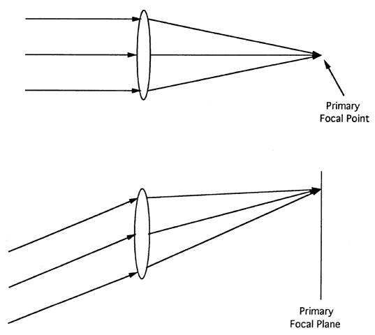
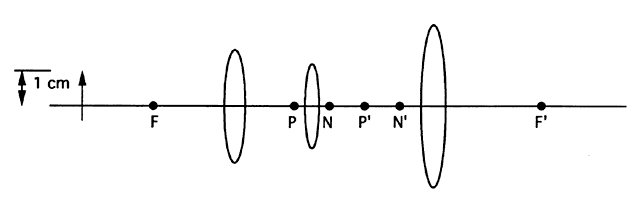
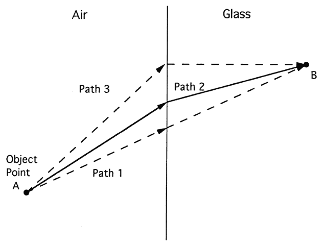
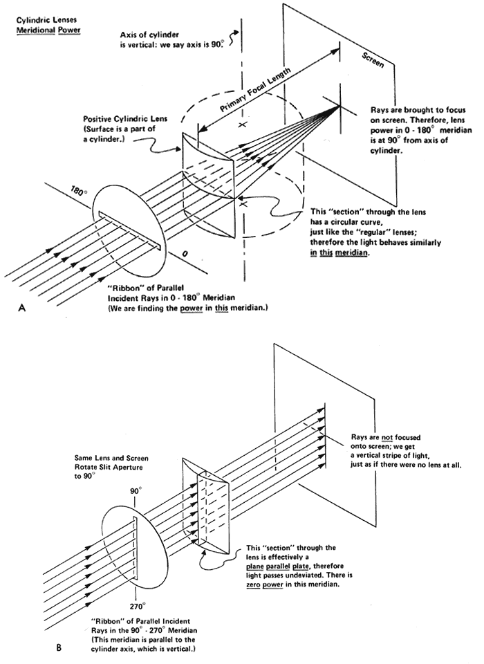
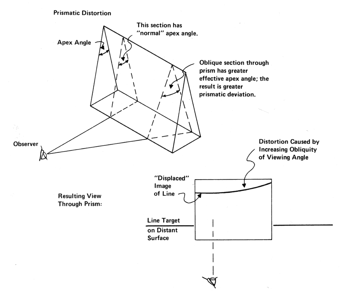
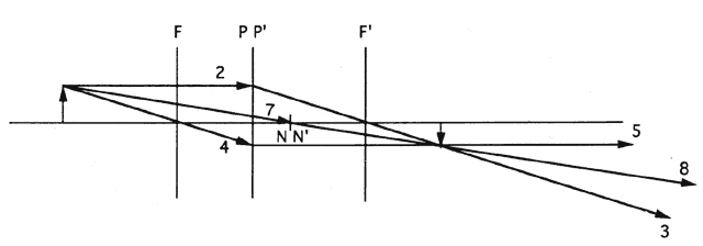
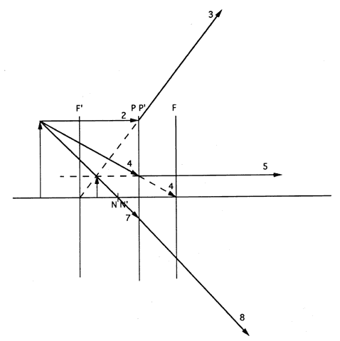
This section discusses some clinical applications of the preceding theory. It is impossible to categorize all the clinical applications of optics.

Pathology of the ocular media can be categorized on the basis of its effect on image formation. There are three general classes of pathology: opaque lesions, scattering or contrast-reducing lesions, and aberration-producing lesions.

Examples of opaque lesions include granular stromal dystrophy of the cornea, asteroid hyalosis, and some types of congenital cataract. The important clinical point is that opaque lesions do not affect vision unless the pupil is almost completely obscured or unless the lesion is very 
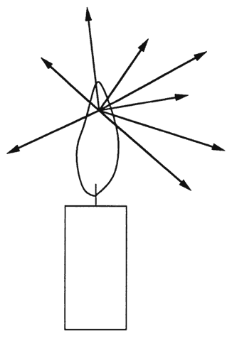
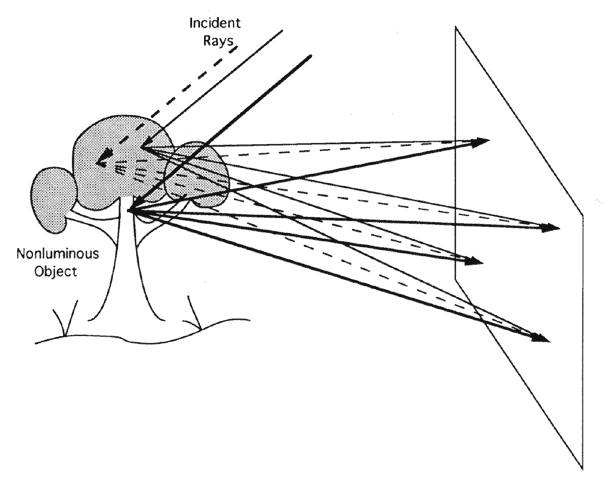
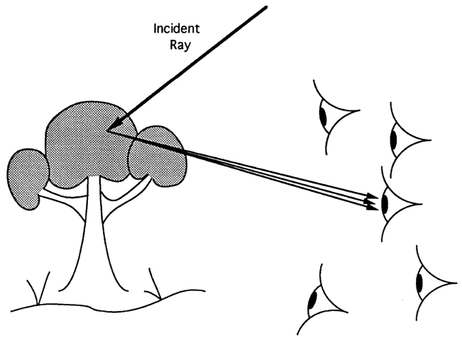
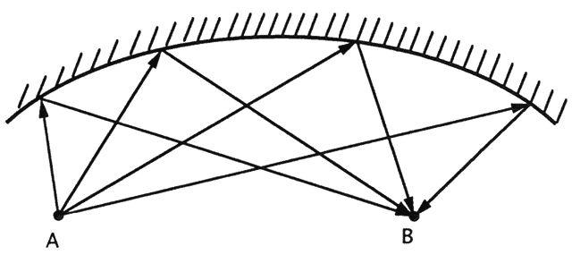
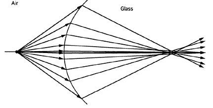
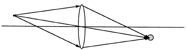
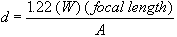
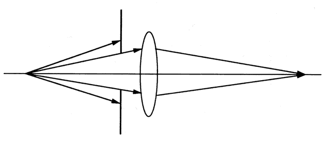
close to the retina.

Place a piece of opaque tape in the center of a trial lens and image a candle. The central obscuration has little effect on the image. Light from each object point completely fills the lens (Fig. 81). A small opaque lesion blocks some of the light, but most still passes through the lens. The light that does traverse the lens is still redirected to produce a one-to-one correspondence between object and image. At most, an opaque lesion produces a small decrease in image brightness, which, as discussed previously, is barely noticeable.

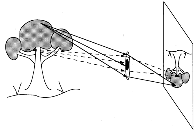
Fig. 81. An opaque lesion blocks some light, but light traversing the unaffected part of the lens still forms an image. The image is slightly dimmer, but otherwise unaffected.

Opaque lesions are usually quite apparent on slit lamp exam but may coexist with other subtler pathology. Problems can arise if visual symptoms are inappropriately attributed to opaque lesions. For example, a patient with a crescent-shaped iris remnant on the lens (from an old posterior synechia that was broken) presents with an arcuate scotoma. The scotoma seemed to correspond to the shape of the iris remnant, which was assumed to be the cause of the scotoma. Two years later, the patient presented with advanced field loss and elevated intraocular pressure (IOP), and the diagnosis of primary open-angle glaucoma was finally made.

When the patient initially presented, it would have been easy to constrict the pupil so that the iris covered the remnant on the lens, and to retest the visual field. If the scotoma had still been present, then it clearly was not caused by the iris remnant. Unfortunately, simple maneuvers 
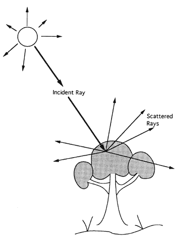
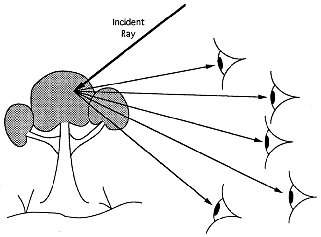
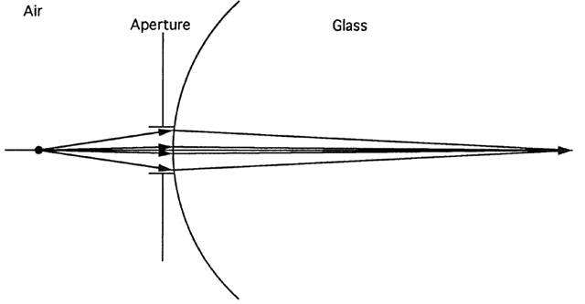
for diagnosing optical problems are often overlooked.

Typical scattering lesions include vitreous hemorrhage, posterior capsular cataract, and corneal edema. Light striking the abnormal area of the media is not blocked as in opaque lesions. Light traverses the lesion but is scattered in the process. The scattered light distributes generally over the entire retina (Fig. 82). Light that passes through the normal parts of the ocular media still creates an image on the retina, but the image is washed out by the scattered light. The effect is similar to raising the house lights during a movie, only more pronounced. Generally, vision is markedly affected, and these are the easiest lesions to diagnose. Patients complain of rainbows, halos, and glare.

Fig. 82. Scattering lesions partially disrupt the one-to-one correspondence between object and image by distributing some light randomly over the image. Light that traverses the unaffected part of the lens still produces an image, but the contrast is somewhat washed out.

Typical aberration-producing lesions include keratoconus, aphakia, subluxed lenses, and postkeratoplasty astigmatism. As discussed, light from a point source is distributed over a small region of the image instead of being confined to a perfect point. Provided the light is spread over only a small area, visual acuity is high. Aberration-increasing lesions cause light from a point source to spread over an abnormally large area and may cause the light distribution to become asymmetric.

Patients with these problems often have near normal acuity but complain of distinct visual phenomena. For example, spectacle-corrected aphakes characteristically complain of pincushion distortion (doorways curve in the middle, appearing too thin to pass through). The visual complaint may be quite variable, depending on the cause of the aberration. Keratoconus patients may complain of a variety of different phenomena because each cone is a different shape and produces different aberrations. The essential feature is not any aspect of the vision per se but rather that the patient is able to describe in vivid detail the visual experience. The visual complaint is specific, not vague. The patient can often draw on paper the appearance of a point source, and this often gives a clue to the problem.

For example, patients post radial keratotomy (RK) may complain of “seeing” the incisions. It was not until RKs were performed with small numbers of incisions that it became clear that the “incisions” the patient was “seeing” and the corneal incisions were not in the same meridians. For instance, if the patient had a four-incision RK with cuts in the 180 and 090 meridians, the patient reported the “incisions he or she saw” in the 045 and 135 meridians. Moreover, some patients “saw” the incisions even when the pupil was much smaller than the optical zone.

The patient cannot be seeing the incisions. If the incisions are opaque, they do not affect the image. If the incisions scatter light, then the contrast is diminished, but this does not cause the patient to see lines in specific meridians. In fact, the patient does not see the incisions 
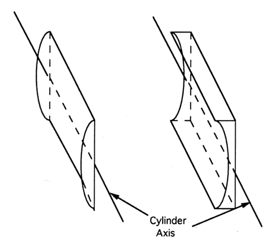
at all. The cornea retracts between the incisions, creating four cylinders with axes in the meridians between the incisions (Fig. 83). These cylinders create the aberrant image that gives the mistaken impression that the patient is “seeing the incisions.”

Fig. 83. A representation of the corneal surface after a four-incision radial keratotomy. The incisions are in the valleys. The corneal tissue retracts between incisions, causing the peaks that produce a “fourfold” form of astigmatism.

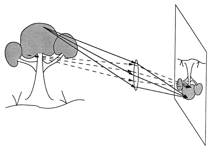
The importance of apertures is often overlooked. First, it is impossible to selectively “look through” only part of the pupil. Consider a patient with good acuity despite a dislocated intraocular lens (IOL) with a positioning hole in the center of the pupil. The question is often asked, “Which part of the pupil is the patient looking through?” The answer is “all parts.” Light from an object point fills the pupil, and some passes through the IOL, some through the positioning hole, and some through the empty pupil. The patient will see well if there is enough light focused on the retina to yield an adequate image despite decreased contrast and possibly glare from the optic's edges. If the patient does see well, it is not because he or she is looking through only the IOL.

Vision is preserved until late in the course of granular dystrophy because the lesions are opaque and do not affect the retinal image until the pupil is nearly totally obscured. However, some explain the preservation of vision by assuming that the patient is somehow “pinholing” by selectively looking through a small part of the cornea between opaque lesions. If the patient were pinholing, then he or she would have an unusually large depth-of-focus, and this could be demonstrated. Patients with granular dystrophy do not exhibit increased depth-of-focus until late in the disease when the pupil becomes nearly a single pinhole.

Of course, it is possible to move the eye so that one looks through only a segment of a bifocal or trifocal spectacle. The eye moving independently of a spectacle, or even a contact lens, can arrange its relatively small pupil so that all the light passing through the pupil passes through only one spectacle segment. The distinction between a bifocal spectacle and a bifocal (or multifocal) IOL is important. At any one time, a patient looks through either the distance or near segment of a spectacle, so all the light on the retina is focused for either near or far. However, with a bifocal IOL, light is always split between two different images simultaneously. There is always some in-focus and some out-of-focus light on the retina.

The importance of the pupil in regulating retinal light levels is often overstated. From dawn to high noon, the amount of ambient illumination varies by thirteen orders of magnitude. The area of the pupil changes by, at most, two orders of magnitude. The pupil may help compensate for small transient fluctuations in illumination, but other mechanisms, such as retinal adaptation, are much more important than the pupil for adjusting to the large variation in light levels that we are exposed to in the course of a day.

Many factors besides light level influence pupil size, indicating that the pupil has other roles than simply regulating retinal illumination. For instance, the pupil constricts during accommodation. Clearly, this is not to regulate retinal illumination, but it does increase depth-of-focus 
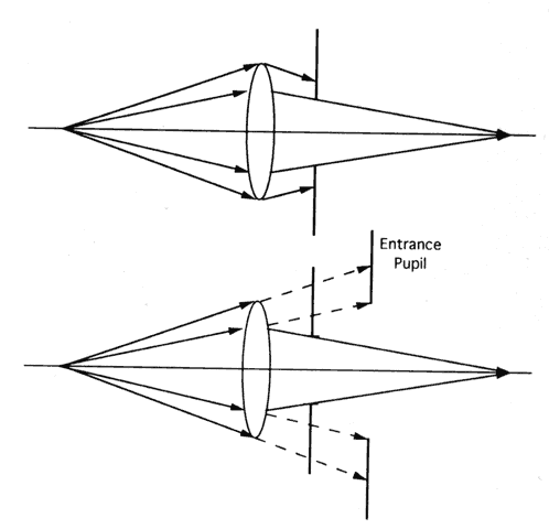
and decrease spherical aberration.

The pupil is also an important consideration in the prescription of visual 
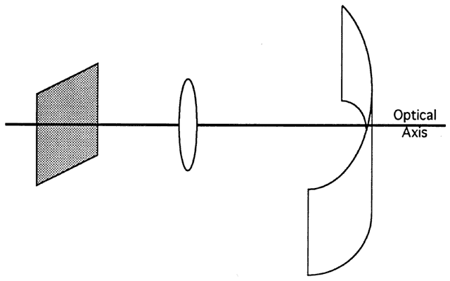
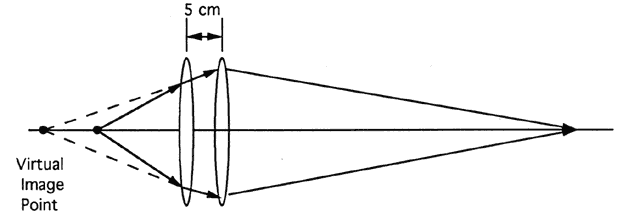
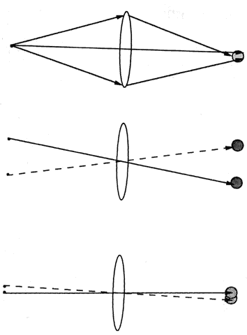
aids. Two important considerations are magnification and illumination. Galilean telescopes produce upright images and are shorter than Keplerian telescopes, making them attractive as a spectacle-mounted visual aid. However, the exit pupil is inside the telescope (Fig. 84). Because of this, some of the light emerging from the exit pupil of the telescope misses the eye's entrance pupil. Thus, some of the light entering the telescope is wasted, and the retinal illumination suffers.

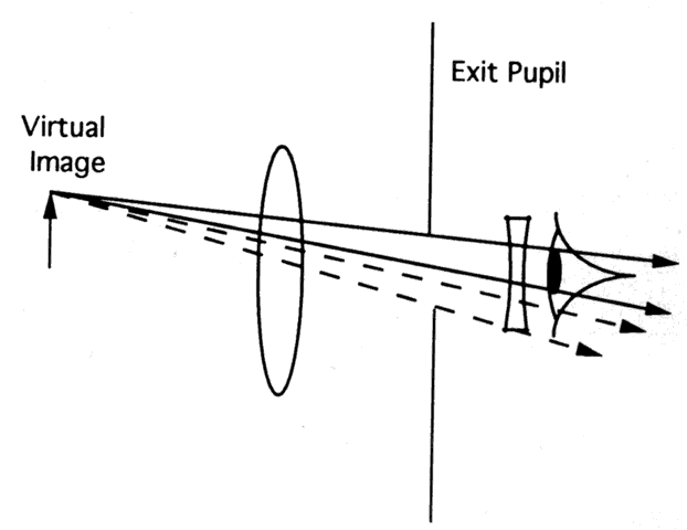
Fig. 84. In a typical Galilean telescope, the aperture stop and entrance pupil are the edges of the objective lens. Thus, the exit pupil is inside the telescope. Some of the light leaving the telescope necessarily fails to enter the observer's eye (dotted lines) and is wasted.

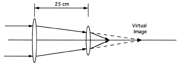
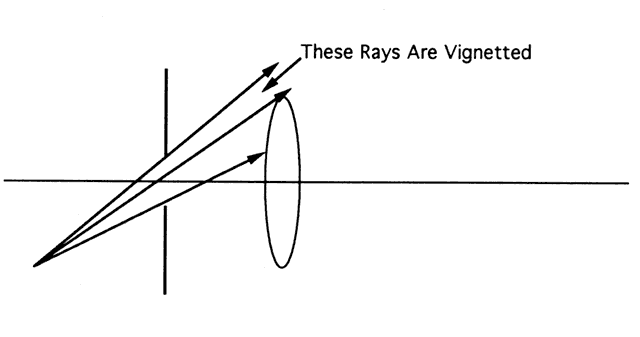
The Keplerian telescope is longer than the Galilean and heavier because it must contain a prism assembly to erect the image that would otherwise be inverted. These aspects make it unsuitable for a spectacle-mounted visual aid. However, the exit pupil is behind the second lens (Fig. 85), so the user may place the exit pupil of the telescope in the entrance pupil of his or her eye. Essentially all the light from the telescope enters the eye. When a patient requires both a bright and enlarged image, a hand-held Keplerian telescope may be the best choice.

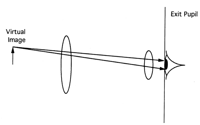
Fig. 85. In a typical astronomical telescope, the aperture stop and entrance pupil are the edges of the objective lens. Thus, the exit pupil is behind the telescope. Most of the light leaving the telescope enters the observer's eye.

It is well known that miosis decreases the visual field. In theory, the small pupil should decrease the general retinal illumination but not alter the field. The decrease in field size is caused by the so-called cosine drop-off law. The beam of light from off-axis points that reaches the retina has a smaller cross-sectional area than the beam from on-axis points (Fig. 86). Thus, less light from off-axis points reaches the retina. The visual field is defined by the point where the amount of light reaching the retina falls below threshold. The smaller the pupil, the smaller the field.

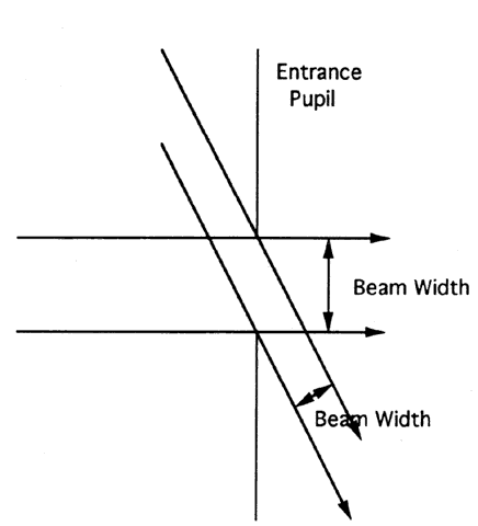
Fig. 86. The beam of light entering a system from off-axis points is much narrower than that from on-axis points.

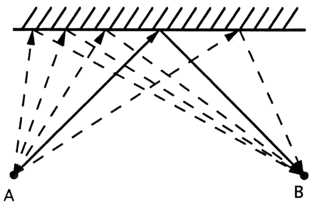
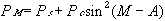
Pupils play an important role in ophthalmoscopy. Direct ophthalmoscopy is like looking into a room through an old-fashioned keyhole. The view is limited (Fig. 87). The field-of-view can be enhanced by placing a lens in the keyhole to form an image. This is the principle of indirect ophthalmoscopy, and the fundus camera. Indirect ophthalmoscopy may be done binocularly or monocularly. Thus, the essential distinction between direct and indirect ophthalmoscopy is not binocularity. In direct ophthalmoscopy, the observer directly views the retina. In indirect ophthalmoscopy, the observer views an image of the retina.

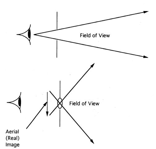
Fig. 87. The view through an external aperture may be quite limited. Placing a lens in the aperture and viewing the resulting image increases the view.

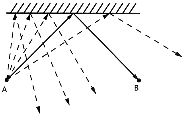
In both types of ophthalmoscopy, the retina must be illuminated. The illumination and viewing paths should be separate, or light reflected from the cornea obscures the retinal image. Binocular ophthalmoscopy divides the pupil of the eye under examination into three parts. Illumination enters through one part, and each eye of the examiner views the retina through another part (this arrangement is referred to as dark field illumination). The headpiece of the indirect ophthalmoscope contains two periscopes that effectively shrink the examiner's interpupillary distance so that both examiner's eyes can peer through separate parts of the patient's pupil.

The size of the retinal image in indirect ophthalmoscopy depends on the power of the condensing lens. The lower the lens power, the larger the image. Examination of the disc is enhanced by the increased axial magnification that accompanies a larger transverse magnification. Because axial magnification increases as roughly the square of the transverse magnification, some examiners use a + 14.00 D instead of the standard + 20.00 D 
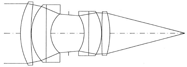
lens to examine the disc for cupping.

Other chapters describe the optics of devices commonly used in clinical practice. The effective use of these instruments requires a knowledge of their operating principles.

Back to Top
ACKNOWLEDGMENTS
The author thanks Roland V. Shack, Ph.D., for his technical advice on aberration theory, fourier optics, image evaluation, and optical testing.

Back to Top

Appendix: Mathematical Development
The mathematical details of geometrical optics are illustrated here by example. The discussion is detailed enough that it should be easy to generalize the results.

Back to Top

SINGLE, POSITIVE, SPHERICAL REFRACTING SURFACE

Consider a spherical refracting surface separating air (n = 1.000) and spectacle crown glass (n = 1.523 at wavelength 587.5618, which is the helium d-line). The refracting surface is spherical and has a radius of curvature (ROC) of 52.3 mm. Locate the image of an object 25 cm in front of the vertex (Fig. 88).

Fig. 88. An optical system consisting of a single positive refracting surface, and the equivalent system in terms of the cardinal points.


RAY SKETCH

Step 1: In this case, the principal planes overlap and are both located at the vertex. The nodal points also overlap and are both located at the center of curvature. The focal points are found by first calculating the power. The paraxial power is calculated from:

The primary focal point is nair/+ 10.00 D = 10.00 cm in front of the vertex. The secondary focal point is nglass/+ 10.00 D = 15.23 cm behind the vertex. The cardinal points are shown in Figure 88.

Steps 2 through 8: These are illustrated in Figure 89.

Fig. 89. Ray sketch of the system. The rays are numbered according to the steps described in the text.


VERGENCE CALCULATION

The object's reduced vergence is -4.00 D (= -1.00/ 0.25 m). The image's reduced vergence is + 6.00 D. The image is real because the image vergence is positive. The image distance is 1.523/6.00 = 25.38 cm. The transverse magnification is -4.00/6.00 = -2/3. The image is inverted and reduced.

EXACT RAY TRACE

Consider the ray shown in Figure 90. With use of trigonometric analysis, which is beyond the scope of this text, this ray is found to intersect the surface at exactly 0.9725 mm behind the vertex and 1.00389 cm above the axis. The angle of incidence is found to be 13.35712°. From this, Snell's law gives:

Fig. 90. An exact ray trace takes into account the curvature of the surface and uses Snell's law to determine the exact light path, which differs slightly from that predicted by paraxial optics. Details are in the text.

1.000(sin 13.35712)=1.523 sin R

Thus, the angle of refraction, R, is 8.72472°.

This ray intersects the optical axis at 24.64543 cm behind the vertex. Note that according to the vergence calculation, the ray should intersect the axis 25.38 cm behind the vertex. The exact calculations show that this ray is actually some 7.3 mm in front of the position predicted. Why?

The exact ray trace was performed with a ray that was not close enough to the axis to qualify as a paraxial ray. Vergence calculations are paraxial calculations only.

Back to Top

SINGLE, NEGATIVE, SPHERICAL REFRACTING SURFACE

The situation is exactly the same as in the previous example except that the surface is concave instead of convex (see Fig. 90). Note that the focal planes are “reversed” (i.e., the secondary focal plane is in front of the lens and the primary focal plane is behind the lens). Also, the nodal points are in front of the lens.

RAY SKETCH

The ray sketch is shown in Figures 91 and 92.

Fig. 91. An optical system consisting of a single negative refracting surface, and the equivalent system in terms of the cardinal points.

Fig. 92. Ray sketch for the system in Figure 91. The vertical scale is expanded for clarity. The image is upright, virtual, and reduced.


VERGENCE CALCULATION

The object's reduced vergence is -4.00 D, the image's reduced vergence is -14.00 D. The image is virtual because the image vergence is negative. The image distance is 1.523/-14.00 D = -10.88 cm or 10.88 cm in front of the secondary principal plane. The transverse magnification is -4.00/-14.00 = 0.29. The image is upright and reduced. Notice that reduced vergence still applies even though the image is in front of the refracting surface.

EXACT RAY TRACE

Just as in the previous example, an exact ray trace would show that the actual rays do not perfectly converge at the image.

Back to Top

POSITIVE THIN LENS, SAME MEDIUM ON BOTH SIDES OF THE LENS

Consider a thin equiconvex lens fabricated from borosilicate crown glass number 7 (n = 1.517 at the helium d-line). Each surface has an ROC of 10.34 cm (+ 5.00 D). The lens is in air (Fig. 93).

Fig. 93. A single, positive, thin lens in air. Note that the principal points and nodal points all coincide.


RAY SKETCH

Although physically the lens has two surfaces, optically the lens is thin so it can be represented by a single surface. As in the case of a single refracting surface, the principal planes coincide. The difference between this and the previous examples is that the nodal points coincide with the principal points. The ray sketch is shown in Figures 93 and 94.

Fig. 94. Ray sketch of a single, positive, thin lens in air.


VERGENCE CALCULATION

The object's reduced vergence is -4.00 D. The image's reduced vergence is + 6.00 D. The image is real because the image vergence is positive. The image distance is 1.00/6.00 D = 16.67 cm behind the secondary principal plane. The transverse magnification is -4.00/6.00 = -2/3. The image is inverted and reduced.

Back to Top

POSITIVE THIN LENS, DIFFERENT MEDIUM ON EACH SIDE

This situation is identical to the previous example except that the medium on the image side is changed to water (n = 1.333). This changes the power of the second lens surface to 1.517 - 1.333/0.1034 = + 1.78 D. The lens now has a power of + 6.78 D.

RAY SKETCH

The secondary focal plane is 1.333/+ 6.78 D = 19.66 cm behind the secondary principal plane. The primary focal point is 1.000/+ 6.78 D = 14.75 cm in front of the primary principal plane. The principal planes still coincide. The two nodal points coincide with each other (i.e., N and N' are in the same location). However, unlike the previous example, the nodal points and principal points do not coincide (Fig. 95). The nodal points are displaced. The distance between the primary principal plane and the primary nodal point (PN) always equals the distance between the secondary principal plane and the secondary nodal point (P'N'). The difference between the primary focal length (f) and the secondary focal length (f') equals the distance between principal and nodal points. To summarize:

Fig. 95. Ray sketch of a single, positive, thin lens, air in front of the lens and water in back.

PN = P'N' = f' - f

The ray sketch is shown in Figure 95.

VERGENCE

The object's vergence is -4.00 D. The image's vergence is + 2.78 D. The image is real. The image distance is 1.333/2.78 D = 47.95 cm. The transverse magnification is -4.00/2.78 = 1.44. The image is inverted and enlarged.

Back to Top

NEGATIVE THIN LENS, SAME MEDIUM ON EACH SIDE

Compared with the analogous example of the positive thin lens, the only difference is the reversal of the primary and secondary focal planes. The ray sketch is shown in Figure 96.

Fig. 96. Ray sketch of a single, negative, thin lens in air. The vertical scale is enlarged for clarity.

Back to Top

NEGATIVE THIN LENS, DIFFERENT MEDIUM ON EACH SIDE

Compared with the analogous example of the positive thin lens, the major difference is the reversal of the primary and secondary focal points, and the nodal points are displaced in front of the lens. The ray sketch is shown in Figure 97.

Fig. 97. Ray sketch of a single, negative, thin lens, air in front of the lens and water in back. The vertical scale is enlarged, and the object distance is increased to 35 cm for clarity.

Back to Top

POSITIVE THICK LENS IN AIR

Consider a thick lens fabricated from spectacle crown glass (n = 1.523 at 587.5618 nm, the helium d-line). Let the front surface have an ROC of 10.46 cm (power = + 5.00 D) and the back surface have an ROC of 13.075 cm (power = + 4.00 D). Let the center thickness be 6.92 mm (Fig. 98).

Fig. 98. A positive thick lens in air (top). The principal planes for each individual surface (middle). The reduced system (bottom).


GAUSSIAN REDUCTION

The first step in dealing with this system is to reduce it to an equivalent system with only one pair of principal planes. This is called gaussian reduction. The total power of the combined system (D) is given by:

Where D1 = power of the first surface, D2 = power of the second surface, and n2 = refractive index of the glass.

The distance between the primary principal plane of the front surface and the primary principal plane of the combined system (designated as P1P) is given by:

Where t = lens center thickness and n1 = index of medium in front of first surface.

The distance between the secondary principal plane of the second surface and the secondary principal plane of the system (designated as P'2P') is:

Where n3 = the refractive index of the medium behind the second surface.

For this specific case,

The negative sign indicates that the system's secondary principal plane is to the left of the second surface's secondary principal plane.

The focal length is 1/+ 8.92 D = 11.2 cm.

RAY SKETCH

Once the reduced system is obtained, the ray sketch is fairly straightforward. A ray sketch for an object 25 cm in front of the primary principal plane is shown in Figure 99. The essential difference between this and previous examples is that now the principal planes do not overlap. Rays intersecting the primary principal plane emerge from the secondary principal plane at the same distance from the optical axis, but in a different direction (unless they go through the nodal points). Rays that go through the nodal points have the same direction but are displaced.

Fig. 99. Ray sketch for a positive thick lens with the same medium on both sides.


VERGENCE CALCULATION

The vergence calculation is similar to the others. Note that the object and image distances are measured with respect to the primary and secondary principal planes, respectively, and not with respect to the lens surfaces.

Back to Top

NEGATIVE THICK LENS IN AIR

For comparison, let this be the same lens as in the previous example except with concave instead of convex surfaces.

GAUSSIAN REDUCTION

Using the same formulas given above,

The situation is illustrated in Figure 100.

Fig. 100. A negative thick lens in air (top). The principal planes for each individual surface (middle). The reduced system (bottom).


RAY SKETCH

This is shown in Figure 101. It is analogous to a negative thin lens in air except for the space between the principal planes.

Fig. 101. Ray sketch for a negative thick lens in air.

Back to Top

POSITIVE THICK LENS IN WATER

Consider the positive thick lens example except with water instead of air in front of the lens. The power of the front surface changes to + 1.82 D.

GAUSSIAN REDUCTION

The total power is

RAY SKETCH

The ray sketch is shown in Figure 102.

Fig. 102. Ray sketch for a positive thick lens with water in front.

Back to Top

NEGATIVE THICK LENS IN WATER

This is the same negative thick lens above except with water in front. The front surface power decreases to -1.82 D.

GAUSSIAN REDUCTION

The total power is given by:

The position of the primary principal plane is given by:

RAY SKETCH

The ray sketch is similar to the negative thick lens in air except that the nodal points are displaced from the principal planes and the focal lengths differ (Fig. 103).

Fig. 103. Ray sketch for a negative thick lens with water in front.

Back to Top

CALCULATING THE CRITICAL ANGLE FOR TOTAL INTERNAL REFLECTION

When light moving in a high-index medium strikes an interface with a lower index medium, the light may pass through the interface or may be internally reflected. Whether the light is transmitted or reflected depends on the angle of incidence and the refractive indices of the two media. For any two media there is a critical angle given by the formula:

Back to Top

VECTORS

A vector is an abstract mathematical representation for anything that has both magnitude and direction. Two vector quantities are routinely used in clinical practice, namely, cylinders and prisms. To prescribe a cylinder, both a power (magnitude) and an axis (direction) must be specified. Similarly, to prescribe a prism, both a power (magnitude) and base position (direction) must be specified. In contrast, to prescribe a sphere, only a power (magnitude) must be specified; there is no direction.

Vector arithmetic is a set of rules developed by mathematicians to perform operations such as addition and subtraction of vectors. Vector arithmetic is quite different from ordinary arithmetic, and one can be led far astray if intuitive notions based on ordinary arithmetic are applied to vectors. To give a concrete example, suppose you walk 4 miles due east, turn, and walk 3 miles due north. Ordinary arithmetic tells us that you have walked a total of 7 miles, but vector arithmetic tells us that you are only 5 miles (as the crow flies) from the original starting point.

Fortunately, it is not necessary to understand the rules of vector arithmetic to use vectors effectively. Moreover, the rules of vector arithmetic are well summarized in many textbooks and thus will not be repeated here. The interested reader can find an excellent treatment in a paper by Jaffe and Clayman.1

Clinicians need not master the mathematical details; they should appreciate that prisms and cylinders add (and subtract) vectorially. For example, suppose one wants to use prisms in a patient with a combined deviation of 3Δ right hypertropia and 4Δ esotropia. It would be correct to prescribe 3Δ base down OD and 4Δ base out OS. However, it is expensive to grind prism into a lens, and because the prism power is low, it might be better to put the correction into a single lens. Vectors can be used to determine the appropriate prism power and base position (5Δ base at 217).

The vector “calculation” can be done graphically by use of a ruler, protractor, and graph paper. Base-up prism and base-down prism can be represented by vectors pointing straight up and straight down, respectively. For the right eye, base in and out are represented by vectors pointing left and right, respectively. For the left eye, base in and out are represented by vectors pointing right and left, respectively.

Specify a point on the graph paper as the starting point or origin, and choose an appropriate scale--in this case, perhaps one prism diopter to the inch. Starting at the origin, draw one of the vectors, say the 4Δ base out vector (Fig. 104). Next, starting at the end of the first vector, draw the second vector representing 3Δbase down (see Fig. 104). Finally, draw a vector from the origin to the end of the second vector. The length of this line is the final prism power, and the angle this line makes with the horizontal gives the orientation of the base. If done with care, this is a very accurate way of adding vectors.

Fig. 104. Vectors can be used to graphically determine the single prism equivalent to two prisms with different orientations.

As a second example, suppose a patient has 6Δ of prism OS base at 30°. What is the combined deviation? First, draw the vector on the graph paper. From the end of the vector, extend a vertical line to the horizontal axis and a horizontal line to the vertical axis. The length of these horizontal and vertical lines gives individual prisms (Fig. 105).

Fig. 105. Vectors can also be used to determine the equivalent horizontal and vertical deviations produced by a single prism oriented at an oblique axis.

Vectors can also be used to calculate the net spherocylindrical power produced by two cylinders (at oblique axes) in contact. Occasionally, refractions are performed by using trial clips placed on a pair of existing spectacles to hold additional trial lenses. If the patient requires only a change in spherical power, it is easy to calculate the new prescription by adding the power of the spherical trial lenses to the existing prescription. However, if the patient requires a change in cylinder axis, it can be difficult to calculate the new prescription because the cylinder in the trial clip will usually be at an oblique axis to the spectacle's cylinder.

One way around the problem is to directly measure the spectacles with trial lenses still in place using a lensmeter to determine the net spherocylindrical power. Anyone who has tried this finds that it can be difficult to accurately neutralize the combination, especially if the optical axis of the spectacle lens does not coincide with that of the trial lenses. Alternatively, one could calculate the net power using the methods described by Jaffe and Clayman. Today, preprogrammed calculators or computer software for calculating net power is commercially available. Of course, the whole problem can be side-stepped by not using trial clips.

Doubtless, the majority of clinicians would like to completely avoid dealing with the combination of cylinders at oblique axes. However, today many cataract and refractive surgeons are interested in surgically induced astigmatism, and this often requires adding or subtracting cylinders at oblique axes. The next section illustrates a variety of ways to calculate surgically induced change in corneal power.

Back to Top

CALCULATING SURGICALLY INDUCED CHANGE IN CORNEAL POWER

In general, postoperative K-readings differ from preoperative K-readings. The change in corneal power is often called the surgically induced astigmatism. However, the term surgically induced astigmatism is somewhat misleading because, in general, there is both a spherical and an astigmatic change in corneal power. Consequently, the term surgically induced change in corneal power (SICCP) will be used.

Conceptually, the SICCP is simply the difference between the postoperative and preoperative corneal powers. The difficulty comes in actually calculating the SICCP because this usually involves subtracting spherocylinders at oblique axes. There are several ways to calculate SICCP, and again these will be illustrated by using a specific example.

Consider a patient with preoperative K-readings of 45.00/45.50 at 100; after radial keratotomy the K-readings are 40.00/42.00 at 150. What is the SICCP?

No matter what method is used to calculate the SICCP, a useful first step would be to transpose the K's to standard spherocylinder form (either plus or minus cylinder depending on personal preference). Thus,

Postoperatively: + 40.00 + 2.00 × 060, or + 42.00 -2.00 × 150

Preoperatively: + 45.00 + 0.50 × 010, or + 45.50 -0.50 × 100.

LENSMETER METHOD

An approximate determination of SICCP can be made by use of the lensmeter and trial lenses. First, consider only the cylinder power. If plus cylinders are used, the postoperative cylinder is + 2.00 × 060, and preoperatively it is + 0.50 × 010. To subtract the preoperative cylinder from the postoperative cylinder, select a + 2.00 cylindrical trial lens and place it in a trial frame at axis 150. Then select a -0.50 cylindrical trial lens and place it at axis 010 in the trial frame. Note that a -0.50 lens is used because one wants to subtract the preoperative power from the postoperative power. Be sure to maintain the axis of the -0.50 cylinder at 010 (i.e., change the power but not the axis when subtracting cylinder). Measure the combination in the lensmeter. The author found a power of -0.37 + 2.25 × 072. Note that the combination of two pure cylinders at oblique axes produces some spherical power. Next, subtract the preoperative sphere from the postoperative sphere, obtaining -5.00. Finally, add the sphere to the spherocylinder to give -5.37 + 2.25 × 072 for the SICCP.

Using minus cylinders, one would use -2.00 × 150 and + 0.50 × 100 trial lenses and measure the combination in the lensmeter (+ 0.37 - 2.25 × 162). Subtracting the preoperative sphere from the postoperative gives -3.50. Adding the sphere and cylinder gives -3.12 - 2.25 × 162.

The advantage of the lensmeter method is that it avoids calculation. The disadvantage is that the answer is only approximate, although often it is sufficiently accurate for clinical purposes. For that matter, the K-readings themselves are not perfectly accurate either.

VECTOR GRAPHICAL METHOD

An alternative to the lensmeter that also has the advantage of avoiding calculation but is more accurate is the graphical vector method. In this method, the vector subtraction is performed with ruler, protractor, and graph paper. When vectors are used to represent a cylinder, the vector angle is the axis multiplied by 2, because vector angles vary over a range of 360°, whereas cylinder axes vary over a range of only 180°.

The first step is to select a convenient scale. In this case, 1 diopter equals 2 inches is suitable (for greater accuracy it is best to use a large scale). The vector representing a + 2.00 × 060 cylinder would be 4 inches long and make an angle of 120° with the horizontal (Fig. 106). The vector representing -0.50 × 010 is drawn at the end of the first vector at an angle of 200° with the horizontal (to graph vectors representing negative powers, add 180° to the angle--e.g., 10 × 2 + 180 = 200°). The resultant is found by drawing a vector from the origin to the end of the second vector (+ 2.15 × 067).

Fig. 106. Vectors used to determine the cylindrical component of SICCP.

The induced sphere is found by making use of an important principle. Whenever two spherocylinders in contact add (or subtract), the spherical equivalent of the result is the sum (or difference) of the individual spherical equivalents. Thus, SICCP has a spherical equivalent equal to the postoperative spherical equivalent (41.00 D) minus the preoperative spherical equivalent (45.25 D), or -4.25 D. The sphere is whatever is necessary to produce the correct spherical equivalent--in this case, -5.33 D. The SICCP is -5.33 + 2.15 × 067.

This method also gives only an approximate result. However, when it is performed with some care, the answer is quite close to the exact result.

EXACT CALCULATION

Of course, it is nice to be able to ascertain the exact SICCP. With the ready availability of scientific calculators, it is an easy matter to calculate the SICCP using the following formulas:

Where Pcp = the postoperative cylinder power, Pca = the preoperative cylinder power, Ap = the postoperative axis, and Aa = the preoperative axis.

Where Psp = postoperative sphere, Psa = preoperative sphere, and SICCPc = SICCP cylinder.

These formulas give the exact answer, but they are complicated, and it is easy to make a mistake even when using a calculator. A programmable calculator, or better a computer, can help overcome calculation mistakes. Once the information is programmed, one would only enter the K-readings and immediately get the results.

With the ready availability of computers, there is little need to calculate SICCP using vectors. Nevertheless, vectors continue to be used not as a calculation tool but as a means of succinctly representing SICCP. As a representation of the SICCP, vectors have some drawbacks. Only the cylindrical component of the SICCP can be represented, not the sphere. To refractive surgeons, the sphere can be as important as the cylinder.

The idea of graphing power versus meridian was already introduced as a means of describing cylinders (see Fig. 72). Any spherocylinder can be represented by a graph of power versus meridian, and such graphs indicate both the spherical and cylindrical powers. Thus, power versus meridian graphs provide a complete graphical representation of SICCP.

Graphs of power versus meridian also make it easy to understand how cylinders at oblique axes add (or subtract). When two spherical lenses are placed in contact, their powers add. Similarly, when two spherocylinders are in contact, their powers also add, but on a meridian-by-meridian basis.

The power of a spherocylinder in any given meridian M is given by the formula:

Where PM = power in meridian M, Ps = spherical power, and Pc = cylinder power.

To determine the power in a single meridian produced by two torics in contact, simply add the powers of the individual lenses in the same meridian. Adding powers meridian-by-meridian could be a tedious process, but this can be done with a computer. The graphs of power versus meridian nicely illustrate the interaction of spherocylinders at oblique axes.

Back to Top

REFERENCES

1. Jaffe NS, Clayman HM: Cataract Surgery, 4th ed, Ch 4. St. Louis, CV Mosby, 1991

Back to Top